Roman Kazinnik, Shai Dekel, and Nira Dyn. AbstractâWe present a new image coding algorithm, the geo- metric piecewise polynomials (GPP) method, that ...
IEEE TRANSACTIONS ON IMAGE PROCESSING, VOL. 16, NO. 9, SEPTEMBER 2007
2225
Low Bit-Rate Image Coding Using Adaptive Geometric Piecewise Polynomial Approximation Roman Kazinnik, Shai Dekel, and Nira Dyn
Abstract—We present a new image coding algorithm, the geometric piecewise polynomials (GPP) method, that draws on recent developments in the theory of adaptive multivariate piecewise polynomials approximation. The algorithm relies on a segmentation stage whose goal is to minimize a functional that is conceptually similar to the Mumford–Shah functional except that it measures the smoothness of the segmentation instead of the length. The initial segmentation is “pruned” and the remaining curve portions are lossy encoded. The image is then further partitioned and approximated by low order polynomials on the subdomains. We show examples where our algorithm outperforms state-of-the-art wavelet coding in the low bit-rate range. The GPP algorithm significantly outperforms wavelet based coding methods on graphic and cartoon images. Also, at the bit rate 0.05 bits per pixel, the GPP algorithm achieves on the test image Cameraman, which has a geometric structure, a PSNR of 21.5 dB, while the JPEG2000 Kakadu software obtains PSNR of 20 dB. For the test image Lena, the GPP algorithm obtains the same PSNR as JPEG2000, but with better visual quality at 0.03 bpp. Index Terms—Adaptive nonlinear approximation, image coding, piecewise polynomial approximation, tree-structured segmentation.
I. INTRODUCTION
S
INCE the mid-1980s, there have been many attempts to design “second generation” image coding techniques that exploit the geometry of edge singularities of an image. The reader may consult the survey [25]. Until this day, almost all of the proposed “second generation” algorithms are not competitive with state of the art (dyadic) wavelet coding [26], [28], [32]. In one of the outstanding “second generation” methods [15], Froment and Mallat constructed multiscale wavelet-like edge detectors and showed how to reconstruct a function from the responses of a sparse collection of these detectors. They reported good coding results at low bit rates. There are coding algorithms that are geometric enhancements of existing wavelet transformedbased methods, where wavelet coefficients are coded using geometric context modeling [33]. In a recent work [27], the authors enhance classical wavelet coding by detecting and coding the strong edges separately and then using wavelets to code a residual image. Candès and Donoho [1] constructed curvelets, a bivariate transform designed to provide sparse representations with local multiscale directional information. Do and Vetterli’s construction of contourlets [12] is similar but is a purely discrete Manuscript received April 16, 2006; revised May 2, 2007. The associate editor coordinating the review of this manuscript and approving it for publication was Dr. Giovanni Poggi. R. Kazinnik and N. Dyn are with the School of Mathematical Sciences, TelAviv University, Ramat Aviv, Tel-Aviv 69978, Israel. S. Dekel is with GE Healthcare, Israel. Digital Object Identifier 10.1109/TIP.2007.903250
construction. Cohen and Matei [4] also showed a discrete construction of an edge-adapted transform that is closely related to nonlinear lifting [3]. All of these constructions are redundant, i.e., the output of the discrete transform implementations produces more coefficients than the original input data. The possibility to use these new transforms to outperform wavelet coding is still an ongoing research. LePennec and Mallat [19] recently applied their “bandelets” algorithm to image coding, where a warped-wavelet transform is computed to align with the geometric flow in the image and the edge singularities are coded using 1-D wavelet-type approximations. Previous work that we find to be the closest to ours are the papers by Shukla et al. [29] (see also [24]), Dekel and Leviatan [6], and Demaret et al. [8]. Our approach departs from the framework of harmonic analysis, which is the theoretical basis for transform based methods and even from the more general framework of multiscale geometric processing, and is based on the geometric piecewise polynomials (GPP) method introduced in [18]. The main difference between the GPP algorithm and recent work is that we revisit the “second generation” approach and directly apply segmentation methods. In this respect, there are similarities between the GPP and bandelets algorithm that computes as a first stage the “geometric flow” of the image. However, the bandelets algorithm imposes a “wavelet” structure on the computed geometric flow, while our algorithm applies the conceptually simpler piecewise polynomial approximation scheme. , , the degree of piecewise polynoFor mial approximation error is (1) where
is the collection (2)
and
are triangles with disjoint interiors, such that , and , , are polynomials . We note that there are computational of total degree variants of piecewise polynomial approximation where the domains are polygonal and satisfy a nesting property (see, e.g., [6] and [17]). In comparison, our approach can be regarded a “higher order” method, since the domains over which eventually polynomial approximation is performed, can have “curved” portions [see Fig. 1(b)]. It is known that in the univariate case, wavelets, and piecewise polynomials have the same (theoretical) performance, since their corresponding approximation spaces are identical [11]. However, in the multivariate case, this is no longer true
1057-7149/$25.00 © 2007 IEEE
2226
IEEE TRANSACTIONS ON IMAGE PROCESSING, VOL. 16, NO. 9, SEPTEMBER 2007
Fig. 1. Pruning of a small width Gaussian zero-crossing of the Cameraman image. (a) Overlay of the image gradient and the zero-crossing. (b) Pruned segmentation.
and at least theoretically, piecewise polynomials outperform wavelets whenever the approximated function has some “structure,” i.e., edge singularities that are smooth in some weak sense [7], [17]. We now highlight three key concepts of our GPP algorithm. First, we model an image as a piecewise smooth bivariate function with curve singularities of weak type smoothness. We apply a segmentation algorithm derived from the -functional of [7]. We then approximate the detected edge singularities, where the distortion is resolved with bands and address the inefficiency of polynomial approximation of smooth functions over nonconvex domains. II. GPP ALGORITHM A. Outline of the GPP Algorithm The steps in our coding algorithm are derived from the theory detailed in [7]. Given an image, we first apply the segmentation algorithm of Section II-B that captures the significant edges in the images. Given a target bit rate, segmentation portions are then pruned using the -functional model. The remaining curve segments are then encoded using the lossy adaptive algorithm of Section II-C, which is closely related to adaptive piecewise polynomial curve approximation. In Section II-D, we describe how the segmentation curves are allocated some width, so that they become “bands.” To better fit the -functional model, we apply further partitioning of the segmentation domains. This step, detailed in Section II-E, is almost a “pure-geometric” domain partitioning recursive algorithm, that the decoder can apply without requiring too much information from the encoder. In Section II-F, we give details of the last step of the algorithm where polynomial approximation, quantization and coding are performed over each of the subdomains. In the last step of the algorithm, the decoder reconstructs “band” pixel values by linear interpolation between the values at the two closest pixels to it, in the two subdomains on both sides of the band. The steps of the GPP algorithm are illustrated using the test image Lena in Figs. 4–6.
to the -functional introduced in [7]. For the sake of completeness, we recall a simple form of the -functional and also show its relation to the well known Mumford–Shah functional. In [22] and [23], Mumford and Shah describe an approach for segmenting a bivariate function in order to obtain a “compact” representation for functions having some lower dimen, as in Fig. 1(b), sional structure. Take any partition of , defined by continuous curves , each of finite length, denoted by . The curves may intersect only at endpoints. Thus, the curves partition the into open subdomains, , image domain . be such that , , Let where is the Sobolev space equipped with the seminorm (3) Then, for any gauge
and
, define the energy
(4) which is the error of the approximation of by , combined with two penalty terms, one measuring the piecewise smoothness of and the second, the total length of the segmentation curves of . The Mumford–Shah functional seeks to minimize and piecewise smooth functions , (4) over all partitions control the balance between approxiwhere the weights , mation, smoothness, and the “amount” of geometry one expects in the minimizing solution. We now attach to each curve a weight and we say that the partition is in if . Advancing towards the -functional, a modified version of the Mumford–Shah functional can be expressed as the infimum of
(5) Comparing (4) with (5), we see that the main difference between and lies in the different notion of the lower dimensional “structure.” The energy gauge uses only the length as a measure of lower dimensional structure and does not distinguish for example between a straight line and a circle, both of the same length. Obviously, from an approximation theoretical point of view, the circle is more complex. is defined as The -functional of order
B. Segmentation Into Subdomains of Smoothness The first step of the GPP algorithm is a segmentation procedure whose goal is to approximate the partition corresponding
(6)
KAZINNIK et al.: LOW BIT-RATE IMAGE CODING
2227
Fig. 2. (a) Smooth function over a nonconvex domain, (b) best L quadratic polynomial approximant (PSNR = 21:5 dB), and (c) approximation significantly improves after partitioning (PSNR = 33 dB).
where
measures the (weak-type) smoothness of the segmentation curves, and
(7) measures the (weak-type) smoothness of the surface pieces. , the quantity is For a curve small if the curve is smooth, for example, if the -norm of its second derivative is small. It is also small if the curve is only piecewise smooth, with a “small” number of pieces and it is [10] identically zero for a line segment. The quantity is small if is smooth in and is identically zero if the function is a bivariate polynomial of degree in . The reader should have in mind the case where for a sufficiently small , the curves , of a near-optimal partition , align on the curve singularities of the function, and where over the segmen, the function is smooth. The novelty of the tation domains, -functional is the way it combines the smoothness gauges of the curve and surface to give a geometric generalization of the classical -functional. More importantly, in [7] it is shown that, is equivalent to the roughly speaking, the quantity approximation error defined in (1). Therefore, since a segmentation which is a near-minimizer of (6) leads to a construction of a good piecewise polynomial approximation, we may conclude that designing an algorithm that tries to find such a segmentation is the key to good performance of our coding algorithm. This task is still an ongoing research project; however, for the purpose of low-bit rate coding, we found out that the following simple and heuristic algorithm works sufficiently well. First, we apply the well known Gaussian zero-crossing segmentation algorithm, also known as the “Laplacian–Gaussian” (LoG), with a relatively small width, , of the Gaussian kernel (see, e.g., [16, Section 9.4]). The idea here is to pick out the edge singularities of the image that are not noise or high-frequency texture, which indeed, the Gaussian kernel, smoothes out sufficiently well.
One of the main properties of the zero-crossing algorithm is connectivity, i.e., the segmentation pixels combine to form continuous segmentation curves. Observe, that in correlation segmentation produces smooth with the -functional the segmentation curves that approximate wiggly edge singularities. In Fig. 1, we see the segmentation produced at this initial step. Our next step, which corresponds to the minimization of the -functional, is to prune the collection of segmentation curves. The goal is to identify and remove the non significant portions of the curves and to quantize and encode only the “significant” segmentation pixels. To this end, we subdivide the segmentation curves to short curve segments of fixed “length” (we used 50 pixels in most of our experiments). We then prune away the curve segments where the norm of the image gradient is below some threshold, since these curve portions do not represent significant edges of the image. After that, we sort the remaining curve portions based on their smoothness, using the following formula:
which is a simplification of a “curve smoothness” term appearing in (6). Thus, we prune away the curve portions whose relative higher curvature impact the -functional the most and equivalently, whose encoding requires a higher bit allocation budget. In Fig. 1(a), we see the initial segmentation of the Cameraman image and, in Fig. 1(b), the most “significant” segmentation portions that survived the pruning process. As can be seen, after the pruning, we are left with a “quasi-segmentation” into subdomains with open contours and “cracks.” Obviously, the amount of pruning relates to the target bit rate, we wish to achieve in our coding algorithm. The pruned segmentation can serve as a good basis for coding of geometric images, for example, graphic-art images that are simple piecewise constant with spline edge singularities. At this stage of the algorithm, two main issues still need to be dealt with. First, we have not fully taken into account the minimization of “surface smoothness” term in (6). Also, after pruning we are left with a “quasi-segmentation” with open contours. These two problems are solved by the partitioning step detailed in Section II-E.
2228
IEEE TRANSACTIONS ON IMAGE PROCESSING, VOL. 16, NO. 9, SEPTEMBER 2007
C. Approximation and Encoding of the Pruned Segmentation Once we have computed the pruned segmentation of Section II-B, we need to efficiently encode it. Recall that the second generation methods [25] did not fully succeed in solving this problem and, therefore, were not able to compete with the more conventional transform-based image compression algorithms. First, we approximate the pruned segmentation by downsamas the maximum error of pling it. We fix a parameter the approximation in pixel distance. Choosing a small gives a very good approximation to the segmentation curves, but leads to a higher bit budget. We downsample the pruned segmentation at the rate and generate its lower resolution, as shown in Fig. 4(c). Observe that, from this downsampled segmentation, we can reconstruct the original “jaggy” segmentation [see Fig. 5(a)] with a maximal error of . After the downsampled segmentation is decoded, it is upsampled back to the original resolution of the image and smoothed using cubic spline least squares approximation [see Fig. 5(b)]. The downsampled segmentation pixel locations are encoded using a high order chain coding algorithm [16], [21] where each downsampled segmentation curve is represented as a starting point and a sequence of travel directions. In our algorithm, we encode the location of the next pixel in the curve, by encoding one of eight possible directions from the previous point (see [9] for a simpler lossy version). We use arithmetic coding combined with context modeling, where each context is determined by the previous four neighbors or equivalently, previous three travel directions. In some sense, this is equivalent to predicting the next point by extrapolating a cubic curve segment that interpolates the previous four points. The lossy curve encoding of [2] obtains on average a bit rate of 1.3 bit/(curve point) with an maximal error of 1 pixel, whereas we would like to have the possibility to go beyond that, i.e., to lower bit rates at the cost of higher errors (typically 2–4 pixels). Our multiresolution approach employs the 8-connected contour encoding at different scales and obtains, on average, a bit rate of 0.1–0.3 bit/(curve point) (see also [20]). In practice, we found that the downsampling factor of the original segmentation is proportional to bit rate of the encoded downsampled segmentation. D. Creating the Segmentation Bands The main goal of bands is to deal with the distortion introduced by the segmentation approximation (downsampling). The concept of bands also appears in [34] and [19], where the authors justify the bands by claiming that the edges in real-life images are “…most often ill-defined…” Indeed, we fix this by allocating some width to the segmentation curves computed in Section II-B, thereby creating bands around edge singularities of the image. First, the bands’ width size in pixel distance, , is computed from two previous parameters: , the Gaussian window width of Section II-B and , the curve approximation error of Section II-C. If these two parameters are small, then we allocate small width to the bands and visa versa. from a reconWe then mark each pixel whose distance is structed segmentation pixel as a band pixel. In our algorithm, the values at band pixels are never encoded, since they are in the vicinity of an edge singularity, whose exact location is unknown to the decoder. Instead, for any band pixel, the decoder
Fig. 3. Budget allocation of the three components in the three images: Eggmean, Cameraman, and Lena.
reconstructs the pixel value by linear interpolation between the decoded values at the two closets pixels in the two subdomains on both sides of the band. Fig. 5(c) shows an example for bands and Fig. 6(c) shows a rendering of the pixel values at band pixels computed by the decoder by interpolating values at neighbor “inner” pixels. E. Convexity Driven Binary Tree Partitioning of the Segmentation Subdomains The purpose of this step is to improve the segmentation of Sections II-B and II-D by further partitioning of the domains into “almost convex” subdomains. In principal, this step complements Section II-B that did not fully take into account the functional (6). Also, recall that the pruning of the segmentation portions in II-B created open contours that we should attempt to reconnect using a method that is very cost effective from the viewpoint of rate-distortion optimization. We now review the basics of the underlying theory that motivates this step. It is known from the theory that the error in polynomial approximation over multivariate domains is determined by both the smoothness of the function and the domain’s geometry. Evidently, it is difficult to approximate a nonsmooth function by low-order polynomials, but it is also difficult to approximate a smooth function over a highly nonconvex domain (see the following example). denote the multivariate polynomials Let (order ). Given a bounded domain , of total degree we define the degree of polynomial approximation of a function by (8) As the next result shows, polynomial approximation over convex domains is well characterized by the classical -functional (7). and functions Theorem 2.1: For all convex domains [5] (9) depends on and . Whenever the domain is not where convex, (9) becomes (10) where the constant on the right hand side of the inequality further depends on the geometry of the domain. Indeed, in Fig. 2(a), we see a function that is very smooth in an open ring-shaped domain. We claim that for this domain the right hand side constant
KAZINNIK et al.: LOW BIT-RATE IMAGE CODING
2229
Fig. 4. (a), (b) Pruning of the initial segmentation of Lena, notice the sorting out of the jagged edges; (c) 1-D approximation employs downscaling, before lossless encoding.
Fig. 5. (a) Shows the “jaggy” reconstruction (upscaling) after decoding, (b) smoothing prediction is subsequently applied to produce smooth curves out of the “jaggy” reconstruction, and (c) adding bands to the decoded lossy segmentation of (b).
in (10) is large. Indeed, as we see in Fig. 2(b), a quadratic polynomial approximation of this function is of poor quality. When we partition the domain into two “more-convex” domains, the approximation significantly improves [Fig. 2(c)]. This is well understood, since polynomials are smooth function over the entire plane. Thus, equipped with the understanding that “convex is good” when the approximation tool at hand are the classical polynomials, we apply a convex driven binary partitioning algorithm. The algorithm recursively subdivides the segmentation subdomains we get from Section II-C, until they are partitioned into “more convex” subdomains with a satisfactory polynomial approximation. Since the binary partitions need to be encoded, it is advantageous that the partitioning algorithm be pure geometric. Then, at each step of the recursive partitioning, if the decoder receives a “subdivide” bit from the encoder, for a given subdomain, it uses the decoded approximated segmentation, and applies a pure-geometric subdivision algorithm without any further information from the encoder. This is closely related to the dyadic square partitioning, that is widely used in many works. For example, in [29], once the decoder is “informed” by the encoder that a dyadic square must be subdivided, it immedi-
ately knows that it must be subdivided into four smaller dyadic squares. Here is the algorithm description. Given a planar open domain , we denote its convex hull as and the complement to . Notice that the subset contains the convex hull as a number of disjoint connected components, which we denote . For each connected component let as :
where with the collections of all curves in with end points , . Let be the two points where this maximum is attained. The algorithm consists of two steps. First, we select the component having the largest value . Second, we find a point such that and subdivide the in the direction normal to the domain by a ray cast from boundary. For example, the partition of Fig. 2(c) is computed using this method. Furthermore, let us consider for example the case of a “cracked” convex domain, i.e., an open convex domain from which a curve segment with one end point at the boundary
2230
IEEE TRANSACTIONS ON IMAGE PROCESSING, VOL. 16, NO. 9, SEPTEMBER 2007
Fig. 6. (a) Initial domains of smoothness, (b) the final partition obtained with the convex-based dyadic partitioning, (c) its corresponding polynomial approximation, and (d) the linear interpolation at the bands.
Fig. 7. Comparison of artifacts in one region of the Cameraman image for GPP and JPEG2000. (a) JPEG200 coding at 0.05 bpp. (b) JPEG2000 coding at 0.10 bpp. (c) GPP coding at 0.05 bpp. (d) Original region.
Fig. 8. R-D performance comparison of the GPP algorithm and JPEG2000 for the Chess, Cameraman, and Lena real-life images.
and one internal end point, was removed. In this case, will have one connected component and the point will be the internal end point of the “crack.” See [13] for more details and examples. Therefore, we see that this step “corrects” a previous step where segmentation portions were pruned away and attempts to “reconnect” these portions with linear lines, at minimal cost in term of bit rate, with the goal of creating subdomains over which the quality of polynomial approximation should improve substantially. For each of the two new subdomains, we compute the polynomial approximation (explained in Section II-F) and if the approximation error is greater than some predefined threshold, we proceed to recursively subdivide the corresponding subdomain. The encoder writes a single bit to the bitstream notifying the decoder whether to subdivide a domain. In practice, we observed
that it is worthwhile to test the first three “least convex” components, i.e., the components with largest , and chose the one that minimizes the approximation error the most. In this variant, one needs to encode two bits per subdivision. As can be seen in Fig. 3, the binary space partition (bsp) information encoded in this stage, is relatively small fraction of the total bit allocation budget. F. Polynomial Approximation and Quantization in the Subdomains of Smoothness In each subdomain, created at Section II-E we compute of the target funca low-order polynomial approximation tion using the least-squares technique. The degree of the polynomials is fixed for all domains. To ensure stability of the quantization of the polynomial’s coefficients, we first compute a repin an orthonormal basis of . resentation of
KAZINNIK et al.: LOW BIT-RATE IMAGE CODING
2231
Fig. 9. Artificial and real-life images coding examples with J2K (JPEG2000) versus GPP. One can observe in (k)–(l) and (o)–(p), where J2K and GPP encoded with the same bit rate and PSNR, that GPP obtains perhaps better visual quality. Notice how GPP improves the coding of geometry as the bit rate increases. (a) The artificial Eggmean [14]. (b) J2K coding at 0.01 bpp, PSNR = 24:4 dB. (c) GPP coding at 0.01 bpp, PSNR = 29:7 dB. (d) The real-life chess. (e) J2K 0.08 bpp, 15 dB. (f) GPP 0.08 bpp, 20.7 dB. (g) J2K 0.15 bpp, 22 dB. (h) GPP 0.12 bpp, 22 dB. (i) J2K 0.05 bpp, 19.94 dB. (j) GPP 0.046 bpp, 21.5 dB. (k) J2K 0.07 bpp, 21.6 dB. (l) GPP 0.07 bpp, 21.6 dB. (m) J2K 0.015 bpp, 23.65 dB. (n) GPP 0.015 bpp, 24 dB. (o) J2K 0.030 bpp, 26 dB. (p) GPP 0.030 bpp, 26.1 dB.
For example, in the case of bivariate linear polynomials, this simply amounts to transforming the standard polynomial basis using a Graham–Schmidt process to an orthonormal basis of . This gives a representation , with , 1, 2, 3. Since, at the time of decoding, the decoder has full knowledge of the geometry of , the Graham–Schmidt process is carried out by the decoder in exactly the same way as the encoder. is subsequently quantized and encoded in The polynomial this stable basis. After all of the coefficients , for all the subdomains are computed and quantized, they are encoded separately for each using the well known variable length
coding (VLC) technique, combined with arithmetic encoding. At the decoder, the quantized coefficients of the polynomial are decoded and the polynomial is reconstructed. We note that this algorithm compresses, on average, the representation of each bivariate linear polynomial (determined by three real numbers) to 1.8 bytes. G. Budget Allocation In Fig. 3, we show the relative distribution of the total bit allocation budget for three test images. There are three main components of the encoded data: geometry (pixel chains of downsampled segmentation), polynomials (quantized coefficients in the
2232
IEEE TRANSACTIONS ON IMAGE PROCESSING, VOL. 16, NO. 9, SEPTEMBER 2007
TABLE I R-D PERFORMANCE COMPARISON OF GPP AND JPEG 2000
stable representation), and BSP tree (the BSP tree of the convex driven binary space partitioning algorithm). H. Experimental Results We applied our GPP algorithm to known test images at low-bit rates and compared the performance of GPP to the best wavelet image coding algorithm known to us: Taubman’s Kakadu implementation [31] of the JPEG2000 standard [32]. It should be noted that not all JPEG2000 compression algorithms provide the same coding performance, and, therefore, one should take care and reference the correct JPEG2000 implementation. The GPP algorithm efficiently encodes geometric images, both artificial, and real-life. In Fig. 9, we see that at low bit rates, both the visual quality and rate-distortion performance of the GPP algorithm are substantially superior to JPEG2000. In addition, at low bit rates, the GPP algorithm encodes images with relatively good visual quality and preserves the key geometric features, as can be seen in Fig. 7. Roughly speaking, it is not surprising that the performance of the GPP coding algorithm depends on the amount of “geometric structure” found in the image. We see on the Chess and Cameraman images, that have relatively more “geometric structure” than other real-life images, that the GPP algorithm outperforms JPEG2000 by 5 dB at 0.08 bpp and 1.5 dB at 0.05 bpp, respectively. However, on the Lena image that contains texture elements and a relatively small amount of geometry, the rate-distortion performance of GPP is similar to JPEG2000, with perhaps better visual quality of the GPP algorithm. The R-D comparison experiments are summarized in Table I and Fig. 8, showing that GPP consistently outperforms JPEG2000 in the very low-bit rate. However, the GPP algorithm clearly underperforms JPEG2000 in the high bit rates. In the high-rate part no new edges are added to the segmentation and the encoding inside the subdomains becomes the most crucial. While GPP employs a dyadic partitiong, a more sophisticated encoding in the subdomains is required in the higher bit rates, such as transform based [29], etc. ACKNOWLEDGMENT The authors would like to thank the referees for suggestions and comments that significantly improved the paper. REFERENCES [1] E. Candès and D. Donoho, “Curvelets and curvilinear integrals,” J. Approx. Theory, vol. 113, no. 1, pp. 59–90, 2001. [2] S. Carlsson, “Sketch based coding of grey level images,” Signal Process., vol. 15, pp. 57–83, Jul. 1988.
[3] R. L. Claypoole, G. M. Davis, W. Sweldens, and R. G. Baraniuk, “Nonlinear wavelet transforms for image coding via lifting,” IEEE Trans. Image Process., vol. 12, no. 12, pp. 1449–1459, Dec. 2003. [4] A. Cohen and B. Matei, “Compact representations of images by edge adapted multiscale transforms,” IEEE Trans. Image Process., vol. 1, no. 10, pp. 8–11, Oct. 2001. [5] S. Dekel and D. Leviatan, “The bramble-hilbert lemma for convex domains,” SIAM J. Math. Anal., vol. 35, no. 5, pp. 1203–1212, 2004. [6] S. Dekel and D. Leviatan, “Adaptive multivariate approximation using binary space partitions and geometric wavelets,” SIAM J. Numer. Anal., vol. 43, no. 2, pp. 707–732, 2005. [7] S. Dekel, D. Leviatan, and M. Sharir, “On bivariate smoothness spaces associated with nonlinear approximation,” Constr. Approx., vol. 20, no. 4, pp. 625–646, 2004. [8] L. Demaret, N. Dyn, and A. Iske, “Image compression by linear splines over adaptive triangulations,” Signal Process., vol. 86, pp. 1604–1616, 2006. [9] U. Desai, M. Mizuki, I. Masaki, and B. K. P. Horn, “Edge and mean based image compression,” Tech. Rep., Mass. Inst. Technol., Cambridge, MA, 1996. [10] R. DeVore and G. Lorentz, Constructive Approximation, ser. Grundlehren der Mathematischen Wissenschaften (Fundamental Principles of Mathematical Sciences). Berlin, Germany: Springer-Verlag, 1993, vol. 303. [11] R. DeVore and B. Lucier, “Wavelets,” in Acta Numerica. Cambridge, U.K.: Cambridge Univ. Press, 1992, pp. 1–56. [12] M. Do and M. Vetterli, “The contourlet transform: An efficient directional multiresolution image representation,” IEEE Trans. Image Process., vol. 14, no. 12, pp. 2091–2106, Dec. 2005. [13] N. Dyn and R. Kazinnik, “Two algorithms for approximation in highly complicated planar domains,” in Algorithms of Approximation, A. Iske and J. Levesley, Eds. New York: Springer-Verlag, 2006. [14] G. Elber, Irit Solid Modeler, Technion 1996 [Online]. Available: http:// www.cs.technion.ac.il/~irit [15] J. Froment and S. Mallat, Second Generation Compact Image Coding With Wavelets, C. K. Chui, Ed. New York: Academic, 1992, vol. Wavelets: A tutorial in theory and applications. [16] A. K. Jain, Fundamentals of Digital Image Processing. Englewood Cliffs, NJ: Prentice-Hall, 1989. [17] B. Karaivanov and P. Petrushev, “Nonlinear piecewise polynomial approximation beyond besov spaces,” Appl. Comput. Harmon. Anal., vol. 15, pp. 177–223, 2003. [18] R. Kazinnik, “Image compression using geometric piecewise polynomials,” Ph.D. dissertation, School Math., Tel-Aviv Univ., Tel-Aviv, Israel. [19] E. LePennec and S. Mallat, “Sparse geometric image representations with bandelets,” IEEE Trans. Image Process., vol. 14, no. 4, pp. 423–438, Apr. 2005. [20] J. Lerman, S. Kulkarni, and J. Koplowitz, “Multiresolution chain coding of contours,” in Proc. Int. Conf. Image Processing, Nov. 1994, vol. 2, pp. 615–619. [21] J. Lim, Two-Dimensional Signal and Image Processing. Englewood Cliffs, NJ: Prentice–Hall, 1990. [22] D. Mumford and J. Shah, “Boundary detection by minimizing functionals,” presented at the IEEE Conf. Computer Vision and Pattern Recognition, 1985. [23] D. Mumford and J. Shah, “Optimal approximations by piecewise smooth functions and associated variational problems,” Commun. Pure Appl. Math., vol. 42, pp. 577–685, 1989. [24] H. Radha, M. Vetterli, and R. Leonardi, “Image compression using binary space partitioning trees,” IEEE Trans. Image Process., vol. 5, no. 12, pp. 1610–1624, Dec. 1996. [25] M. M. Reid, R. J. Millar, and N. D. Black, “Second-generation image coding: An overview,” ACM Comput. Surv., vol. 29, no. 1, pp. 3–29, Mar. 1997. [26] A. Said and W. Pearlman, “A new fast and efficient image codec based on set partitioning in hierarchical trees,” IEEE Trans. Circuits Syst. Video Technol., vol. 6, no. 6, pp. 243–250, Jun. 1996. [27] D. Schilling and P. Cosman, “Preserving step edges in low bit rate progressive image compression,” IEEE Trans. Image Process., vol. 12, no. 12, pp. 1473–1484, Dec. 2003. [28] J. M. Shapiro, “Embedded image coding using zerotrees of wavelet coefficients,” IEEE Trans. Signal Process., vol. 41, no. 12, pp. 3445–3462, Dec. 1993. [29] R. Shukla, P. Dragotti, M. Do, and M. Vetterli, “Rate-distortion optimized tree-structured compression algorithms for piecewise polynomial images,” IEEE Trans. Image Process., vol. 14, no. 3, pp. 343–359, Mar. 2005.
KAZINNIK et al.: LOW BIT-RATE IMAGE CODING
[30] D. Taubman, “High performance scalable image compression with ebcot,” IEEE Trans. Image Process., vol. 9, no. 7, pp. 1158–1170, Jul. 2000. [31] D. Taubman, Kakadu Software Toolkit Version 3.0 for JPEG2000 Developers 2005 [Online]. Available: http://www.kakadusoftware.com [32] D. Taubman and M. Marcellin, JPEG2000: Image Compression Fundamentals, Standards, and Practice. Norwell, MA: Kluwer, 2002. [33] M. Wakin, J. Romberg, H. Choi, and R. Baraniuk, A. L. M. Unser and A. Aldroubi, Eds., “Geometric methods for wavelet-based image compression,” in Proc. SPIE Conf. X, 2003, vol. 5207, pp. 507–520. [34] Y. Yomdin and Y. Elichai, “Normal forms representation: A technology for image compression,” Proc. SPIE, vol. 1903, pp. 204–214, Feb. 1993. Roman Kazinnik studied applied math at the Saint-Petersburg Polytechnic Institute, U.S.S.R., and after four years, transferred to The Technion—Israel Institute of Technology, Haifa, Israel, where he received the M.S. degree in computer science in 1998. He currently pursuing the Ph.D. degree at the School of Mathematical Sciences, Tel-Aviv University, Tel-Aviv, Israel. He defines his current interests as numerical methods of approximation and its applications in PDE and stochastic dynamics.
2233
Shai Dekel received the Ph.D. degree in mathematics from the Tel-Aviv University, Tel-Aviv, Israel, in 2000. Presently, he is a Researcher at GE Healthcare, Tel-Aviv, and has a visiting position at Tel-Aviv University. His research interests include approximation theory, harmonic analysis, and their applications in image processing.
Nira Dyn received the B.Sc. degree in applied mathematics from The Technion—Israel Institute of Technology, Haifa, Israel, in 1965, and the M.Sc. and Ph.D. degrees in applied mathematics from the Weizmann Institute, Rehovot, Israel, in 1967 and 1970, respectively. She has been a Professor of applied mathematics at Tel-Aviv University, TelAviv, Israel, since 1984. Her main field of activity is geometric modeling and approximation theory. She has authored more than 130 papers and has participated actively in more than 80 conferences and workshops. Dr. Dyn serves on the editorial boards of the Journal of Approximation Theory and of the journal Computer Aided Geometric Design.