to encode an optimal cut of the BSP tree, i.e., a sparse piecewise polynomial ... given bit target, rate-distortion optimization strategies are used (see also [23]).
Image coding with geometric wavelets Dror Alani*, Amir Averbuch* and Shai Dekel** *School of Computer Science Tel Aviv University Tel Aviv 69978, Israel **GE Healthcare 6 Hamasger St. Or-Yehuda 60408, Israel
Abstract This paper describes a new and efficient method for low bit-rate image coding which is based on recent development in the theory of multivariate nonlinear piecewise polynomial approximation. It combines a Binary Space Partition (BSP) scheme with Geometric Wavelet (GW) tree approximation so as to efficiently capture curve singularities and provide a sparse representation of the image. The GW method successfully competes with state-of-the-art wavelet methods such as the EZW, SPIHT and EBCOT algorithms. We report a gain of about 0.4 dB over the SPIHT and EBCOT algorithms at the bit-rate 0.0625 bits-per-pixels (bpp). It also outperforms other recent methods that are based on ‘sparse geometric representation’. For example, we report a gain of 0.27 dB over the Bandelets algorithm at 0.1 bpp. Although the algorithm is computationally intensive, its time complexity can be significantely reduced by collecting a ‘global’ GW n-term approximation to the image from a collection of GW trees, each constructed separately over tiles of the image.
1
Introduction
The first segmentation-based coding methods appeared in the early 80’s [9, 11]. These algorithms partition the image into geometric regions over which it is approximated using low-order polynomials. Many variations have since been introduced [5, 10, 12, 13, 14, 15, 18, 24, 27] and among them, the BSP based methods [16, 19, 21]. The BSP technique can be described as follows. Given an initial bounded convex domain in R2 , � � such as [0, 1]2, and a function f ∈ L2 [0, 1]2 , the initial domain is subdivided into two subdomains by intersecting it with an hyper-plane. The subdivision is performed to minimize a given cost functional. 1
This partitioning process then proceeds to operate recursively on the subdomains until some exit measure is met. To be specific, we describe the algorithm of [19], which is a BSP algorithm that identifies a compact geometric description of a target bivariate function. For a given convex polygonal domain Ω, the algorithm finds two subdomains Ω� and Ω�� , and two bivariate (linear) polynomials QΩ� and QΩ�� , that minimize �f − QΩ� �2L2 (Ω� ) + �f − QΩ�� �2L2 (Ω�� ) ,
(1)
over all pairs of polygonal domains Ω� and Ω�� that are the result of a BSP of Ω. The goal in [19] is to encode an optimal cut of the BSP tree, i.e., a sparse piecewise polynomial approximation of the original image that is based on the union of disjoint polygonal domains in the BSP tree. To meet a given bit target, rate-distortion optimization strategies are used (see also [23]). Inspired by a recent progress in multivariate piecewise polynomial approximation [7, 8, 3], we enhance the above BSP by what can be described as a geometric wavelets approach. Let Ω� be a child of Ω in a BSP tree, i.e., Ω� ⊂ Ω and Ω� is created by a BSP partition of Ω. We use the polynomial approximations QΩ and QΩ� found by (1) and define ∆
∆
ψΩ� = ψΩ� (f ) = 1Ω� (QΩ� − QΩ ) ,
(2)
as the geometric wavelet associated with the subdomain Ω� and the function f . A reader familiar with wavelets [2, 4] will notice that ψΩ� is a ‘local difference’ component that belongs to the detail space between two levels in the BSP tree, a ‘low resolution’ level associated with Ω and a ‘high resolution’ level associated with Ω� . The geometric wavelets also have the ‘vanishing moments’ property, i.e., if f is locally a polynomial over Ω, then minimizing of (1) yields QΩ� = QΩ = f and therefore ψΩ� = 0. However, the BSP method is highly nonlinear. Both the partition and the geometric wavelets depend on f , so we cannot expect some of the familiar properties of isotropic wavelets like a two-scale relation, biorthogonality or a partition of unity to hold. Our algorithm proceeds as follows. The BSP algorithm is applied to generate a ‘full’ BSP tree P. Obviously, in applications, the subdivision process is terminated when the leaves of the tree are subdomains of sufficiently small volume, or equivalently, in image processing, when the subdomains contain only a few pixels. Under certain mild conditions on the partition P and the function f , we have [3] f=
�
ψΩ (f ),
a.e. in [0, 1]2,
Ω∈P
where ∆
∆
ψ[0,1]2 = ψ[0,1]2 (f ) = 1[0,1]2 Q[0,1]2 .
2
(3)
Once the ‘full’ geometric wavelets BSP tree is constructed, a sparse representation is extracted using the ‘greedy’ methodology of nonlinear approximation. We sort all the geometric wavelets (2) according to their L2 -norm, i.e.,
� � � � � � � � � � � � �ψΩk1 � ≥ �ψΩk2 � ≥ �ψΩk3 � · · · , 2
2
2
(4)
and given an integer n ∈ N, we approximate f by the n-term geometric wavelet sum n � j=1
ψΩkj .
(5)
The sum (5) is, in some sense, a generalization of the classical greedy wavelet n-term approximation (see [4], [26] and references therein). However, unlike classical wavelets, the geometric wavelets are not even a basis of L2 . Nevertheless, their use in adaptive approximation is theoretically justified in [7] and [3]. At the core of our algorithm is the fact that only a ‘few’ geometric wavelet have large norm. The geometric adaptivity of the BSP procedure, in most cases, ensures that the wavelets whose support intersects the edge singularities of the image, is a long and narrow convex domain aligned with the curve singularities. Thus, roughly speaking, there are substantially less significant geometric wavelets than significant classic dyadic wavelets (see examples in [3]). The algorithm encodes two types of information: the geometry of the support of the wavelets participating in the sparse representation (5) and the polynomial coefficients of the wavelet functions. Good coding performance is achieved by careful quantization of the encoded geometry and by combining the greedy approximation (5) with tree approximation and rate-distortion optimization techniques. The GW algorithm is well suited for low bit-rate compression. For example, the test image Lena is encoded at 0.0625 bits per pixel (bpp) with Peak Signal to Noise Ratio (PSNR) of 28.72. This result outperforms the EZW algorithm [22] (27.54), SPIHT (28.38) [20] and EBCOT (28.30) [25]. The compression of the test image Cameraman at 0.0625 bpp achieves PSNR of 22.93. This result outperforms the JPEG2000 Kakadu algorithm [6] by almost 2 dB. The paper has the following structure: in section 2 we give the details of our algorithm and in section 3 we provide experimental results and compare our method with recent state-of-the-art wavelet and ‘sparse geometric representation’ methods.
2
The GW encoding algorithm
The GW encoding algorithm is composed of three major steps: 3
1. Adaptive BSP tree generation. 2. Finding a sparse GW representation. 3. Encoding the sparse GW representation.
2.1
Adaptive BSP tree generation
The BSP tree generation is a recursive procedure that at each step subdivides a convex polygonal domain Ω by a bisecting line. At each step, we compute the optimal bisection that minimizes (1), from a collection of discrete optional lines, where the degree of the polynomials is of a fixed low order. Once the best partition is computed, Ω is subdivided into the corresponding two children subdomains Ω� and Ω�� and the BSP procedure is applied recursively on each of them. In addition, two new nodes are added to the BSP tree, storing the parameters of the bisecting line, the polygons of Ω� and Ω�� and the coefficients of the wavelet polynomials QΩ� and QΩ�� . The recursive procedure is terminated when either the area of the domain Ω is too small (contains only a few pixels) or the approximation error �f − QΩ �L2 (Ω) ,
(6)
is sufficiently small. Figures 1 and 2 show an example of a few levels of a BSP tree.
Figure 1: BSP of the square Ω. Left: The square is partitioned by the line l. Ω0 and Ω1 are the two child subdomains of Ω. Right: Ω0 is partitioned by l0 . Its child subdomains are Ω00 and Ω01 . Ω1 is partitioned by l1 . Its child subdomains are Ω10 and Ω11 .
4
Ω00
m Ω QQQQ QQQ mmm m m QQQ mm m m QQQ mmm QQQ m m v m ( Ω0 C Ω1 C CC CC {{ {{ C CC { { CC CC {{ {{ C { { C C! { { ! }{ }{
Ω01
Ω10
Ω11
Figure 2: BSP tree of the square in Fig. 1. Each tree node corresponds to a unique polygon. The polygons are denoted by Ω, Ω0 , Ω1 , Ω00 , Ω01 , Ω10 and Ω11 .
Since the BSP tree procedure is computationally intensive, we tile the image and the BSP algorithm is applied on each tile separately, thereby creating a BSP forest. Experience shows that the choice of tiles of size 128 × 128 significantly reduces the time complexity of the algorithm but does not reduce its coding efficiency. Fig. 3 demonstrates a tiling of Lena.
Figure 3: Tiling of Lena (512×512) using tiles of size 128×128.
Image tiling has another advantage. The bisecting lines of the BSP scheme are quantized using their normal representation ρ = x cos θ + y sin θ,
(7)
where ρ is the normal distance between the line and an origin point ‘close’ to the subdivided domain and θ is the angle between the line’s normal and x-axis. As we shall see, ρ is bounded by the length of the tile’s diagonal and hence fewer bits are needed when image tiling is applied. In addition, the quantization of the parameter θ is less sensitive when smaller domains are subdivided. 5
The main disadvantage of image tiling is that, at low bit-rates, there are blocking artifacts at the tiles’ boundaries (see Fig. 12), a phenomena known to those familiar with low bit-rate JPEG compression. In addition, there is a possibility that a long, linear portion of a curve singularity, will be captured by several BSPs, one at each tile, whereas, with no tiling, only a single BSP is needed. Since there is no analytic solution to (1), we apply a brute-force search over a finite discrete (quantized) pre-determined set of bisecting lines. For each fixed bisection line, the approximating polynomials are computed by applying a simple least-squares procedure separately on each of the subdomain. Our experiments show that, for low bit-rate coding, it is actually advantageous to use ‘fine’ quantization of the bisecting lines. This is because, at low bit-rates, only a ‘few’ partitioning lines are encoded, the ones that trace linear portions of the most significant curve singularities in the image. It turns out that it is cost-effective, from a rate-distortion perspective, to encode a good approximation of the curve singularities and avoid large approximation errors in their vicinities. We use a similar quantization scheme to [19] and discretize the set of possible bisecting lines by the parameters ρ and θ of the normal representation (7). The size of the quantizations step depend on the ‘size’ of the polygonal domain. In [19], the ‘size’ is defined as the longest side of the domain’s bounding box, but we find this too crude and use the diameter of the bounding box instead. We apply a uniform quantization of the line orientations θ, where the quantization depends on the size of the domain. We then use uniform quantization for ρ, where the quantization depends on θ. For the purpose of quantization, we set the domain’s size to be the smallest power-of-two that is larger than the diameter of the bounding box. Then, the number of line-orientations is ∆
#θ =
min √
2j ≥
M ·N
2j ,
(8)
where M and N are the lengths of the sides of the bounding box. The range of θ is [− π2 , π] as in Fig. 4.
6
Figure 4: Two partitions of the square. Left: Orientation of the normal that is close to − π2 . Right: Orientation of the normal that is close to π.
For this choice of angular range, we do not have to consider negative values for ρ. This is an improvement over the algorithm of [19] where the range of θ is [0, π] and negative values of ρ are allowed. Thus, roughly speaking, we save one bit and use it to increase the quantization range of θ. Due to the range of [− π2 , π], the (uniform) quantization step size of θ becomes ∆
∆θ =
3π , 2 · #θ
(9)
and the discrete set of line orientations for the polygon Ω is θi = i · ∆θ = i ·
3π , 2 · #θ
i = 0, 1, 2, . . ., #θ − 1.
(10)
Next we quantize ρ. As mentioned before, given a domain Ω, the range of ρ is a function of θ. Let (xc , yc ) be the corner of the bounding-box of Ω. Then, the range where ρ takes values [ρmin , ρmax] is computed by
∆
ρmin (θ) = min {(x − xc ) cos θ + (y − yc ) sin θ} ∆
(x,y)∈V
ρmax(θ) = max {(x − xc ) cos θ + (y − yc ) sin θ},
(11)
(x,y)∈V
where V is the set of vertices of the polygonal boundary of Ω and θ is the fixed line orientation. Given a line-orientation θ, the quantization step of ρ is ∆
∆ρ (θ) = max{| cos θ|, | sin θ|}.
(12)
Equation (12) gives the smallest value for a quantization step size that reveals a new set of pixels with each step, as shown in Fig. 5. 7
Figure 5: A quantization step that reveals a new set of pixels. In this case, θ =
π 4
� and ∆ρ (θ) =
1 2.
For each θi in (10) we have ρij = j · ∆ρ (θi ) = j · max{| cos θi |, | sin θi |}, where
j = minj , minj + 1, . . ., maxj
(13)
∆
minj = �ρmin (θi )/∆ρ (θi )�, ∆
maxj = �ρmax (θi )/∆ρ(θi )�.
(14)
Some of the discrete pairs {θi , ρij } given by (10) and (13), respectively, are actually ‘out-of-range’ possibilities. Two examples that illustrate this are presented in Fig. 6. In the left hand side example, the bisecting line passes through the bounding-box but does not pass through the polygon. In the right hand side example, the bisecting line creates a child subdomain with area below the pre-selected threshold. The encoder and decoder take into account only in-range pairs.
8
Figure 6: Two ‘out-of-range’ partitions of a polygon. Left: the bisecting line (dashed) passes through the bounding-box but does not pass through the polygon (bold). Right: one of the child-polygons has area below a pre-selected threshold.
2.2
Finding a sparse GW representation
The full BSP forest, generated in step 1, may contain a large number of GW nodes. Yet, for low bit-rate coding, only few of them (typically 1-4 %) are needed to obtain a reasonable approximation of the image. Therefore, we apply the ‘greedy’ approximation methodology (see [26, 4] for the case of classical isotropic wavelets and Theorem 3.6 in [3] for the anisotropic case), sort the geometric wavelets according to their energy ‘contribution’ (see (4)) and extract a global n-term approximation from the joint list of all the geometric wavelets over all the image tiles. We found that for the purpose of efficient encoding it is useful to impose the additional condition of a tree structure over each image tile [1]. Namely, we require that if a child appears in the sparse representation, then so does the parent. Once a parent is encoded in this hierarchical representation, then we only need to encode the (quantized) BSP line that creates the child. This significantly saves bits when the geometry of the sparse representation is encoded. On the other hand, the penalty for imposing the connected tree structure is not significant, since with high probability, if a child is significant, then so are his ancestors (this assumption is also used in image coding using isotropic wavelets [22, 20]). Fig. 7 illustrates an n-term GW collection whose graph representation includes some unconnected components and Fig. 8 illustrates the final GW tree after the missing ancestors were added.
9
Figure 7: Example of a greedy selection. The GW tree nodes are 1-31. The chosen GW nodes are 1-4,7,13-14,23,27-29.
Figure 8: The final GW-tree with the additional nodes 5,11 and 6 of the missing ancestors.
Finally, we apply a rate-distortion (R-D) optimization process. Instead of encoding an n-term tree approximation, we generate an n + k geometric wavelet tree and then apply pruning-iterations, where at each step the sub-tree with minimal R-D ‘slope’ is pruned until either a total of k nodes is removed from the tree or until some desired rate is achieved. The method is well known and has been applied before in the setting of isotropic wavelets (see [25]) and in ‘sparse geometric representations’ (see the ‘optimum pruning’ in [19]) and in the ‘prune and join’ algorithm of [23]). We omit the details. Empirical results show that this rate-distortion mechanism increases the PSNR by 0.1 dB in some cases.
2.3
Encoding the sparse GW representation
Before the actual forest is encoded, a small header is written to the compressed file. This header contains the minimum and maximum values of the coefficients of the wavelets (see (15)) QΩ participating 10
in the sparse representation. These values are used by the decoder to decode the coefficients (see 2.3.3). In addition, the header contains the minimum and maximum values of the gray levels in the image. The coefficients’ extremal values are encoded with four bytes each and image extremal values with 1 byte each. Therefore, the header size is 3 × 2 × 4 + 2 × 1 = 26 bytes. Due to the fact that the contribution of the root ‘wavelets’ (3) to the approximation is generally high, all of them are encoded. This is similar to the JPEG algorithm, where the DC component of the DCT transform plays the same role and is always encoded. The encoding procedure is then applied recursively for each GW tree root in each image tile. The following steps are performed for each node Ω that is visited in the recursive algorithm: 1. The quantized coefficients of QΩ are encoded using an orthonormal basis representation. 2. The number of children of Ω that participate in the sparse representation (0,1 or 2) are encoded. 3. In case only one child belongs to the sparse representation, we encode (using one bit) which of the two it is. 4. In case at least one of the children belongs to the sparse representation, we encode the BSP line that bisects Ω using the normal representation (7). Once the information associated with Ω is encoded, the recursion is applied only to the children nodes that belong to the sparse representation. The decoder reconstructs the GW forest and generates the approximation to the image by applying (5). 2.3.1
Encoding the tree structure
There are two types of tree-structure information that are needed to be encoded: the number of children of each node and the information that is needed to distinguish between child nodes. The encoding of the tree structure information is different from [19]. There, if the domain is partitioned, then both its children (or at least their siblings) participate in the representation, while in our waveletbased method, we allow the case where one child is significant and the other (with its siblings) is not. As in sparse isotropic wavelets representations (the ‘zero-trees’ of [22, 20]), with high probability a significant node does not have any significant children nodes. Thus, we encode three values using the static Huffman code. The Zero-Children symbol is encoded by ‘1’, the the One-child symbol by ‘00’ and the Two-Children symbol by ‘01’. If the symbol One-child is encoded, then we need to encode an additional bit which indicates to the decoder which of the two children is the significant. To avoid a synchronization problem at the decoder, we impose a consistent order on the children, in the following way: 11
The first-child of a polygon is defined as follows: 1. If the first point of the parent’s polygon exists only in one child then this child is a first-child. 2. Else, the first point of the parent’s polygon exists in both child’s polygons. In this case, the second point of the polygon is examined. The child’s polygon, which contains the second point, is a first-child. Fig. 9 demonstrates two cases of line-partitioning of a polygon. The left figure shows that the first point of the parent’s polygon exists only in one of the child’s polygons, whereas in the right figure the first point exists in both of the child’s polygons.
Figure 9: Two examples for line-partitioning of the polygon ABCDE. Left: the first-child is ABCGF. Right: the first-child is ABCG.
2.3.2
Encoding the bisecting line
As explained in section 2.1, the selection of the bisecting lines in the BSP forest is dictated by the quantization of θ and ρ given by the normal equation (7). Recall also that some of the bisections are considered out-of-range (see Fig.6). The encoding steps are: 1. The number #θ is computed by (8). 2. The index θi , given by (10), is encoded using variable length coding. 3. The range [ρmin , ρmax] is computed using (11). 4. The quantization step ∆ρ (θ) of ρ, is computed by (12). 5. minj and maxj are computed by (14). 12
6. We loop on the indices of ρ in [minj ,maxj ], pruning out the out-of-range pairs [θi , ρi,j ] while counting the number of in-range bisections. The index of the selected bisection in the in-range set is found. 7. The index of the selected bisection is encoded using variable length coding. Observe that steps 1,3,4,5 and the counting of in-range pairs for a fixed θi in step 6, are also performed by the decoder with no need for additional information from the encoder. 2.3.3
Encoding the coefficients of the wavelet polynomials
We now describe how the wavelet polynomials QΩ are encoded. Whereas each bivariate linear polynomial is determined by three real numbers, i.e. by 12 bytes, our algorithm, on average, compresses this representation to 1.5 bytes per polynomial. Here are the main ingredients of the wavelet polynomial encoding algorithm: • The coefficients of the polynomial QΩ are quantized and encoded using an orthonormal representation of Π1 (Ω), where Π1 (Ω) is the set of all bivariate linear polynomials over Ω. • A bit allocation scheme for the coefficients is applied using their distribution function (over all the domains). • We always encode each tile’s ‘root’ wavelet (3). 2.3.4
Quantizing the coefficients in an orthonormal polynomial basis representation
To ensure the staility of the quantization process of the geometric wavelet polynomial QΩ , we first need to find its representation in appropriate orthonormal basis. The orthonormal basis of Π1 (Ω) is found using the standard Graham-Schmidt procedure. Let V1 (x, y) = 1, V2 (x, y) = x and V3 (x, y) = y be the standard polynomial basis. Then, an orthonormal basis of Π1 (Ω) is given by U1 =
V1 V2 − < V2 , U1 > U1 V3 − < V3 , U1 > U1 − < V3 , U2 > U2 , U2 = , U3 = , ||V1 || ||V2 − < V2 , U1 > U1 || ||V3 − < V3 , U1 > U1 − < V3 , U2 > U2 ||
where the inner product and norm are associated with the space L2 (Ω). Let Q ∈ Π1 (Ω). We denote by α, β and γ the coefficients in the representation Q = αU 1 + βU 2 + γU 3.
13
(15)
2.3.5
Bit allocation of polynomial coefficients
Fig. 10 illustrates three histograms of the distribution function of the coefficients (15) of the geometric wavelets participating in a sparse representation of Lena. 25
25
25
20
20
20
15
15
15
10
10
10
5
5
5
0 −2500 −2000 −1500 −1000
−500
0
500
1000
1500
2000
0 −2000
−1500
−1000
−500
0
500
1000
1500
2000
0 −4000
−3000
−2000
−1000
0
1000
2000
3000
4000
Figure 10: Histograms of the polynomial coefficients of Lena. Left: histogram of α. Middle: histogram of β. Right: histogram of γ.
Observe that the distributions of α, β and γ are similar, in the sense that, with high probability a coefficient is small (the graph resembles a Generalized-Gaussian function). Hence, we apply the following bit-allocation scheme. We use four bins to model the coefficients’ absolute value. The bin limits are computed by the encoder and passed to the decoder. For each wavelet polynomial we do the following: 1. We find the bins of the absolute value of the three coefficients. 2. We encode with one bit the event where all three coefficients are ‘small’, i.e. their absolute value is in the bin containing zero. 3. If one of the coefficients is not ‘small’, we encode the bin number of each of the coefficients. Using arithmetic coding one can apply a different context model for each coefficient type, α, β or γ, and therefore adapts to the appropriate distribution function. We observed that Huffman coding also produces similar results. 4. We write to the compressed file, with no further encoding, the quantized bits of the coefficients.
14
2.4
Budget allocation
Fig. 11 shows how the bit allocation of Lena at the bit-rate 0.0625 bits per pixel (bpp) is distributed among the GW algorithm components
Figure 11: Bit allocation distribution for encoding Lena at 0.0625 bpp. The output size is 2·KBytes.
At higher bit-rates, the bit budget for the polynomial coefficients relatively increases, while the bit allocation for the bisecting lines relatively decreases.
3
Experimental results
Fig. 12 presents the reconstructed images of Lena from the GW algorithm at different bit-rates. Note that the algorithm preserves the significant edge singularities of the image, even at very low bit-rates, without the ‘ringing’ artifacts that is a known phenomena of low bit-rate isotropic wavelet coding. However, at the lower bit-rates the boundaries of the 128 × 128 tiles are visible.
15
Figure 12: Top left: original Lena. Top right: 0.25 bpp, PSNR=33.16. Bottom left: 0.125 bpp, PSNR=30.73. Bottom right: 0.0625 bpp, PSNR=28.72.
Table 1 compares between the rate-distortion (PSNR) performance of the GW algorithm and published results of several state-of-the-art wavelet based algorithms on Lena. Table 2 compares between the rate-distortion (PSNR) performance of the GW algorithm and other recent algorithms that are based on ‘sparse geometric representation’, the Prune-Join algorithm of Shukla, Dragotti, Do and Vetterli [23] and the Bandelets of Le-Pennec and Mallat [17]. The
16
Compression ratio
bit-rate (bpp)
GW
EZW [22]
SPIHT [20]
EBCOT [25]
1:64
0.125
30.74
30.23
31.10
31.22
1:128
0.0625
28.74
27.54
28.38
28.30
1:256
0.0315
26.64
25.38
26.1
—
Table 1: Comparison with state-of-the-art wavelet based algorithms on Lena. Entries are in PSNR. algorithm of [23] is very similar in nature to the GW algorithm. Both use partitions of the image over which it is approximated using low order polynomials. However, there are two main differences: the tree structure in [23] is based on dyadic cubes and anisotropic bisecting lines are used only at the leaves of the tree. Also, the underlying approximation scheme in [23] is piecewise polynomials approximation and there is no notion of n-term sums or wavelets. The Bandelets [17] algorithm applies an anisotropic multiresolution transform of the image that is based on a pre-processing step that computes the geometric flow in the image. We note that in the Bandelets algorithm there is an underlying partition of the image into dyadic squares, over which the geometric flow is constrained to be ’unique’, i.e., there is an identification of a single ‘edge’ (if any) within each block. In a way, this is similar to the structure of [23] and perhaps more restrictive than the GW algorithm. Compression ratio
bit-rate (bpp)
GW
Prune tree [23]
Prune-Join tree [23]
Bandelets [17]
1:32
0.25
33.16
32.31
33.01
33.56
1:40
0.2
32.41
30.95
31.98
32.61
1:53
0.15
31.40
29.48
30.86
31.39
1:64
0.125
30.73
—
—
30.63
1:80
0.1
30.00
—
—
29.73
Table 2: Comparison on Lena with ‘sparse geometric representation’ algorithms. Entries are in PSNR. Table 3 shows a performance comparison between the GW, the Kakadu [6] and the SPIHT [20] algorithms on the Cameraman (which perhaps is more ‘geometric’ and hence favorable to our approach). The results reported in Table 3 were obtained by actual runs of the corresponding software. Finally, we present a side-by-side comparison between the GW algorithm and the Kakadu software [6] that implements the EBCOT algorithm [25]. It seems that the Kakadu software performs better than what is reported in [25]. Fig. 13 shows the reconstructed images of Reflect (a ‘graphic’ image), Cameraman and Lena using these two algorithms. Observe that the GW algorithm significantly outperforms Kakadu on ‘graphic’ images. The Kakadu software performs better on Lena. 17
Compression ratio
bit-rate (bpp)
GW
Kakadu [6]
SPIHT [20]
1:32
0.25
27.48
27.29
28
1:64
0.125
25.07
24.11
25
1:128
0.0625
22.93
21.15
22.8
Table 3: Comparison with state-of-the-art wavelet based algorithms on the Cameraman. Entries are in PSNR.
Figure 13: Top left: original Reflect (128 × 128). Top center: Reconstructed Reflect using the GW algorithm, 0.125 bpp, PSNR=30.33. Top right: Reconstructed Reflect using the Kakadu algorithm, 0.125 bpp, PSNR=18.46 Middle left: Original Cameraman (256 × 256). Middle center: Reconstructed Cameraman using the GW algorithm, 0.125 bpp, PSNR=22.93. Middle right: Reconstructed Cameraman using the Kakadu algorithm, 0.125 bpp, PSNR=21.15. Bottom left: Original Lena (512 × 512). 18 Bottom center: Reconstructed Lena using the GW algorithm, 0.0625 bpp, PSNR=28.72. Bottom right: Reconstructed Lena using the Kakadu algorithm, 0.0625 bpp, PSNR=29.24.
4
Conclusions and future work
We presented a new algorithm for image coding that is based on combining the BSP approach with wavelet methodology and uses efficient techniques to encode the sparse geometric wavelet representation of the image. We showed that in the low bit-rate range, the GW outperforms popular waveletbased encoders and recent ‘geometric’ coding algorithms. In the future, better statistical models for the encoding of the BSP geometry and the coefficients of the polynomials should be explored. In particular, we believe that design of new ‘geometric’ context modelling schemes combined with arithmetic encoding, will improve the performance of the algorithm. For example, there are perhaps statistical correlations between parent and child BSP lines. One can also test non-uniform quantizations of the parameters of the normal equation (7) of the bisecting lines, based on the geometry of the domain to be partitioned. Finally, we hope to find new methods to reduce the time complexity of the algorithm.
References [1] A. Cohen, W. Dahmen, I. Daubechies and R. DeVore, “Tree approximation and optimal encoding”, Appl. Comput. Harmon. Anal., vol 11, num. 2, pp. 192-226, 2001. [2] I. Daubechies, “Ten lectures on wavelets”, CBMS-NSF Reg. Conf. Series in Applied Math., Vol. 61, SIAM, 1992. [3] S. Dekel and D. Leviatan, “Adaptive Multivariate Approximation Using Binary Space Partitions and Geometric Wavelets”, SIAM J. Num. Anal., vol. 43, num. 2, pp. 707-732, 2005. [4] R. DeVore, “Nonlinear approximation”, Acta Numerica, vol. 7, pp. 51-150, 1998. [5] A. K .Jain, “Image data compression: A review”, Proc. IEEE, vol. 69, pp. 349-389, Mar. 1981. [6] Kakadu JPEG2000 software V4.5, http://www.kakadusoftware.com/ [7] B. Karaivanov and P. Petrushev, “Nonlinear piecewise polynomial approximation beyond Besov spaces”, Appl. Comput. Harmon. Anal., vol. 15, num. 3, pp. 177-223, 2003. [8] B. Karaivanov, P. Petrushev and R. Sharpley, “Algorithms for nonlinear piecewise polynomial approximation: Theoretical aspects” , Trans. Amer. Math. Soc., vol. 355, pp. 2585-2631, 2003. [9] M. Kocher and M. Kunt, “A contour-texture approach to image coding”, in ICASSP Proc., pp. 436-440, 1982. 19
[10] M. Kunt, M. Benard, and R. Leonardi, “Recent results in high compression image coding”, IEEE Trans. Cir. Syst., vol. CAS-34, no. 1, pp. 1306-1336, 1987. [11] M. Kunt, A. Ikonomopoulos and M. Koche, “Second generation image coding techniques”, Proc. IEEE, vol. 73, pp. 549-574 Apr. 1985. [12] R. Leonardi and M. Kunt, “Adaptive split-and-merge for image analysis and coding”, Proc. SPIE, vol. 594, 1985. [13] H. G. Muzmann, P. Pirsch, and H. Grallet, “Advances in picture coding”, Proc. IEEE, vol. 73, pp. 523-548, Apr. 1985. [14] A. N. Netravali and B. G. Haskell, “Digital Pictures: Representations and Compressions” New York, Plenum, 1988. [15] A. N. Netravali and J. O. Limb, “Picture coding: A review”, Proc. IEEE, vol. 68, pp. 366-406, Mar. 1980. [16] M. S. Paterson and F. F. Yao, “Effcient binary space partitions for hidden-surface removal and solid modeling”, Discrete Comput. Geom., vol. 5, pp. 485-503, 1990. [17] E. L. Pennec and S. Mallat, “Sparse geometric image representations with bandelets”, IEEE Trans. Image Process., vol. 14, num. 4, pp. 423-438, 2005. [18] M. Rabbani and P. W. Jones, “Digital image Compression Techniques”, Bellingham, WA: SPIE Press, 1991. [19] H. Radha, M. Vetterli and R. Leonardi, “Image compression using binary space partitioning trees”, IEEE Trans. Image Process., vol. 5, num. 12, pp. 1610-1624, 1996. [20] A. Said and W. Pearlman, “A new fast and efficient image codec based on set partitioning in hierarchical trees”, IEEE Trans. Circ. Syst. Video Tech, vol. 6, pp. 243-250, 1996. [21] P. Salembier and L. Garrido, “Binary partition tree as an efficient representation for image processing, segmentation, and information retrieval”, IEEE Trans. Image Proc., vol. 9, num. 4, pp. 561-576, 2000. [22] M. Shapiro, “An embedded hierarchical image coder using zerotrees of wavelet coefficients”, IEEE Trans. Signal Process., vol. 41, pp. 3445-3462, 1993.
20
[23] R. Shukla, P. L. Dragotti, M. N. Do and M. Vetterli, “Rate-distortion optimized tree structured compression algorithms for piecewise smooth images”, IEEE Trans. Image Process., vol. 14, num. 3, pp. 343-359, 2005. [24] G. J. Sullivan and R. L. Baker, “Efficient quadtree coding of images and video”, IEEE Trans. Acoustic, Speech and Signal Proc., vol. 36, pp. 1445-1453, 1988. [25] David Taubman, “High Performance Scalable Image Compression with EBCOT”, IEEE Trans. Image Process., vol. 9, num. 7, pp. 1151-1170, 2000. [26] V. N. Temlyakov, “Nonlinear methods of approximation”, Found. Comput. Math., vol. 3, pp. 33-107, 2003. [27] J. Vaisey and A. Gersho, “Image compression with variableblock size segmentation”, IEEE Trans. Signal Process., vol. SP-40, pp. 2040-2060, 1992.
21