time domain to frequency domain using an overlapping transform such as a subband ... codec, was coded using a low bitrate coding using an adaptive gain-.
LOW BITRATE AUDIO CODING USING GENERALIZED ADAPTIVE GAIN SHAPE VECTOR QUANTIZATION ACROSS CHANNELS Sanjeev Mehrotra, Wei-ge Chen, and Kishore Kotteri Microsoft Research, Microsoft Corporation, One Microsoft Way, Redmond, WA, 98052 {sanjeevm,wchen,kishorek}@microsoft.com 8
ABSTRACT
8
xm,4
6
log10 |xs [k]|
log10 |xm [k]|
Audio coding at low bitrates suffers from artifacts due to spectrum truncation. Typical audio codecs code multi-channel sources using transforms across the channels to remove redundancy such as middle (mid) - side (M/S) coding. At low bitrates, the spectrum of the coded channels is truncated and the spectrum of the channels with lower energy, such as the side channel, is truncated severely, sometimes entirely. This results in a muffled sound due to truncation of all coded channels beyond a certain frequency. It also results in a loss of spatial image even at low frequencies due to severe truncation of the side channel. Previously we have developed a low bitrate coding method to combat the loss of higher frequencies caused by spectrum truncation. In this paper, we present a novel low bitrate audio coding scheme to mitigate the loss of spatial image. Listening tests show that the combination of the two low bitrate coding methods results in a audio codec that can get good quality even at bitrates as low as 32kbps for stereo content with low decoder complexity.
4
4
2
2
0 0
0
100
200
k
300
400
500
0
(a) Mid channel 8
200
k
300
400
500
(b) Side Channel xs,4
log10 |ˆ xs [k]|
log10 |ˆ xm [k]|
6
4
4
2
2
0
0
100
200
k
300
400
500
(c) Mid Channel After Quantization
Index Terms— Audio Coding, Vector Quantization
100
8
xm,4
6
0
xs,4
6
0
100
200
k
300
400
500
(d) Side Channel After Quantization
1. INTRODUCTION
Fig. 1. Magnitude of spectrum of mid and side coded channels in log domain. Also shown are vectors which tile the missing portion of the side channel spectrum.
With recent interest in direct delivery of music to mobile phones and satellite radios as well as demand for being able to store larger music libraries on portable devices, there is increasing need for good quality audio at lower bitrates. It is well known that existing codecs such as MPEG II-Layer 3 (MP3) and Advanced Audio Coding (AAC) have significant artifacts when coding stereo content below 128kbps. Typical audio codecs first take the input audio signal and segment it into transform blocks, the size of the transform block being determined by signal characteristics such as whether the signal is transient (using smaller transform block sizes) or stationary (which uses larger transform block sizes). The signal is transformed from time domain to frequency domain using an overlapping transform such as a subband filterbank or modulated discrete cosine transform (MDCT). Then, a channel transform is applied across the audio channels (for example the left and right) to remove redundancy. In the remainder of this paper, we will refer to the original channels as those prior to the channel transform, and the coded channels as those after the channel transform. In typical music sources the left and right channels are strongly correlated and thus have a lot of redundancy. A channel transform such as the mid/side (M/S) transform removes this redundancy. √ The mid channel can be defined as xm [k] = (xl [k] + xr [k])/ 2, where xm [k] is the kth spectral coefficient of the mid channel, and xl [k] and xr [k] are those of the left and right channel. √ The side channel can be defined as xs [k] = (xl [k] − xr [k])/ 2. After the channel transform, the spectral coefficients of the coded channels are quantized and entropy coded. The quantization step size used for each coefficient of each
channel is different and is found by using psychoacoustic modeling to find places where larger quantization noise can be tolerated. At low bitrates, there are fewer bits to encode the signal, and thus large quantization step sizes are used to code many of the coefficients. For example, all channels above a certain frequency are quantized to zero in all the channels. Furthermore, at lower bitrates, some of the coded channels, for example the side channel for stereo sources, are further truncated to improve the coding of the mid channel. After quantization, the spectrum of the coded channels can look like that in figure 1(c)-(d), whereas before quantization it will look like that in figure 1(a)-(b), resulting in a muffled sounding signal with very little spatial image. In all figures which show the spectrum in this paper, we show the log of the magnitude of the spectrum. In [1], we presented a novel audio codec which combined traditional waveform audio coding with a low bitrate coding scheme to create a codec which performed on average as good as the best audio codec at that bitrate, but performed better on some clips. It also had a far lower decoder complexity than other audio codecs of similar quality. This codec used traditional audio coding methods to code some portions of the spectrum. The remaining portion of the spectrum, which was quantized to zero by the traditional waveform codec, was coded using a low bitrate coding using an adaptive gainshape vector quantizer with the adaptive codebook being formed by taking modified and unmodified portions of the spectrum which have already been coded. Although this coding works very well for coding the higher portion of the spectrum when both coded channels are
978-1-4244-2354-5/09/$25.00 ©2009 IEEE
9
ICASSP 2009
If K is the number of entries in the codebook used to jointly code the set of N vectors, the best entry in the codebook is found to be lopt ∈ {0, 1, . . . , K − 1} using search. The decoder simply reconstructs as
truncated beyond a large frequency, it does not perform well at lower bitrates when, for example, the side channel spectrum is being truncated very severely, such as below 8kHz. In such cases, an alternate coding method is needed to reconstruct the spatial image. Existing solutions to solve this problem are along the lines of perceptual stereo coding. In intensity stereo coding [2], for example, a stereo source is only coded as a mono source. The effect of stereo is simply perceptually recreated by applying different scale factors to shape the energy in various bands to get the energy envelope of the two channels correct. This has been generalized in binaural cue coding (BCC) in which audio cues such as interaural level difference (ILD), interaural time difference (ITD), and interaural coherence (IC) are sent as parameters from which a downmixed source (such as a single channel source) is reconstructed to stereo [3, 4]. The reconstruction is done so as to preserve these parameters as in the original. Techniques such as this are used in the parametric stereo coding in the High-Efficiency AAC (HE-AAC) audio codec. In this paper, we present an alternate coding method which performs far better than traditional audio codecs, but performs as good as the best audio codecs such as HE-AAC. However, decoder complexity is found to be lower. The basic idea is similar to that used in [1] in that we use an adaptive gain-shape vector quantizer where the codebook is adaptively formed from portions of the spectrum that have already been coded.
ˆ = UX D1/2 Clopt , X X which results in RXˆ Xˆ ≈ RXX . 3. AUDIO CODING USING GSVQ
In this section we present how generalized adaptive gain-shape vector quantization is used in an audio codec. The encoder first encodes the audio signal using a traditional waveform audio codec. For transform blocks where there is strong correlation between the left and the right channels, the traditional audio codec uses mid/side channel coding. For transform blocks where there is not strong correlation, the traditional codec will use left/right stereo coding. In those blocks where left/right stereo coding is used, we simply use the ideas presented in [1] to code the spectrum. In transform blocks which use mid/side channel coding, the original spectrum shown in figure 1(a)-(b) can look like that in figure 1(c)-(d) after quantization using a traditional audio codec at low bitrates. The mid and side channels are both truncated, with the side channel severely truncated. To fill in the missing portion of the spectrum in the mid channel, we can use ideas from [1]. Then the mid channel will look similar to that in figure 1(a). If we inverted the channel transform and reconstructed the left and right channels at this point, we would not get a muffled sounding signal, since the spectrum is full bandwidth. However, due to the side channel spectrum truncation, we would still get a signal with the spatial image lost at most of the frequencies. However, we cannot use the ideas from [1] to fill in the missing portion of the spectrum in the side channel as there is only a small portion of the spectrum that is available to form a codebook. In order to form an effective codebook to code the side channel, we could use portions of the spectrum from the mid channel to augment it. Although this can work, it will only accurately represent the energy of the side channel. Other statistics such as the cross correlation between the two channels will not be preserved. Cross-correlation is also an important statistic to preserve in order to create an accurate stereo image, at least in the lower frequency range. For this we use ideas from section 2. Consider dividing up the missing portion of the side channel spectrum into M non-uniform size vectors as shown in figure 1(b). Similarly divide this portion of the spectrum in the mid channel as shown in figure 1(a). Let these vectors be xm,i and xs,i for the ith vector for the mid and side channels respectively, where i = 0, 1, . . . , M − 1. For example, the i = 4 vector is shown in figure 1. The ith vector simply consists of the original spectral coefficients and can be written as
2. GENERALIZED GAIN SHAPE VECTOR QUANTIZATION Gain shape vector quantization (GSVQ) is a modified version of vector quantization (VQ) that can be used when it is important to preserve the energy of the vector. For example, if the vector x is to be x coded using VQ, then we can write x = �x� �x� , where the first term s = �x� is the gain and the second term y = x/�x� is a unit norm vector. Now, the gain s can be quantized separately using some number of bits so that the gain is more accurately represented. The shape y is a unit norm vector which can be coded using a codebook with unit norm vectors. Although GSVQ allows for better preservation of the energy (or gain) of a vector, it still is not able to control the cross-correlation across two vectors which is important when coding two vectors consisting of spectral coefficients, one from the left channel, and another from the right channel. For example, one of the cues in binaural cue coding is related to cross-correlation [3, 4]. Here we generalize the concept of gain-shape vector quantization across any arbitrary number of vectors. Consider that N vectors, xn , n = 0, . . . , N − 1, have to be coded and we wish to be able to accurately represent the energy and cross- correlation of the vectors. Then we can form a matrix X = [x0 x1 . . . xN−1 ], which has a correlation matrix given by RXX = X∗ X, where X∗ is the Hermitian transpose of the matrix. Then we can code a sufficient number of parameters to represent the symmetric matrix RXX . Now since RXX is symmetric, we can write RXX = UX DX U∗X , where DX is a diagonal matrix, and UX is an orthonormal matrix. Then, if −1/2
Y = DX
U∗X X,
xm,i = [xm [S[i]] xm [S[i] + 1] . . . xm [S[i] + L[i] − 1]]T ,
(4)
where S[i] is the starting position of the ith vector, L[i] is the length of the vector, and xm [k] is the kth spectral coefficient of the mid channel. We can similarly define the vector xs,i , with S[i] and L[i] being the same for both channels for all i. Define the matrix Xi as
(1)
then the matrix Y = [y0 y1 . . . yN−1 ] consists of vectors yn which are of unit norm and uncorrelated. That is RY Y = Y ∗ Y = I, the identity matrix. Instead of coding each vector yn independently using a codebook, we code yn jointly using a codebook where each entry l in the codebook is a matrix which is a set of N vectors cn,l , where Cl = [c0,l c1,l . . . cN−1,l ] satisfies C∗l Cl = I.
(3)
Xi = [xm,i xs,i ],
(5)
which is a L[i]x2 dimensional matrix. Now we can use ideas presented in section 2 with N = 2 to code this matrix. That is, we can code RXX = X∗i Xi for this matrix, then normalize the matrix using equation 1 to obtain Yi and then code Yi using a codebook with entries which satisfy equation 2.
(2)
10
8
8
c4,0,1 c4,0,0 c4,0,2 c4,0,3
6
log10 |x⊥ m [k]|
log10 |xm [k]|
4
4
2
2
0 0
nel domain to left-right original channel domain. Once the inverse transform is applied the spectrum does not have missing spectral coefficients, however, it does have an incorrect spectrum past the truncation point of the side-channel. We code the portion of the spectrum with missing spatial image using the generalized adaptive gain-shape vector quantization presented in section 2. First, we divide this portion of the spectrum of the left and right channels into vectors as shown in figure 3. Define xl,i and xr,i to the left and right ith vectors similar to equation 4. Define the matrix Xi = [xl,i xr,i ] to be the matrix to code similar to equation 5. We code RXX and send it in the bitstream for each i. The normalized matrix Yi is coded using the same codebook formed from the mid channel as described. One simplification is to note that not all components of the matrix RXX need to be sent and thus we can save bits used to code this matrix. The matrix is symmetric so only N (N + 1)/2 components are unique. If the spectrum x is complex, then N of these parameters are real and N (N + 1)/2 − N are complex. The complex parameters can be coded using polar coordinates as magnitude and phase, with phase being more coarsely quantized. Also since we already have some information on the spectrum, we don’t need to send all of these parameters. For example, in the two √ channel case, the mid channel is given by xm,i = (xl,i + xr,i )/ 2 and thus x∗m,i xm,i = (x∗l,i xl,i + x∗r,i xr,i )/2 + Real(x∗l,i xr,i ). Since the mid channel spectrum is already coded, if we know x∗l,i xl,i and x∗l,i xr,i , we can compute x∗r,i xr,i without actually sending any parameters. In general, suppose that the codec uses a channel transform B to code the signal as Z = BX, and then suppose that some of these coded channels are being quantized to zero. Let Z0 be the portion that is not quantized to zero, and let Z1 be the portion that is quantized to zero. That is, RZZ = Z∗ Z = B∗ X∗ XB, where � ∗ � Z0 Z0 Z∗0 Z1 RZZ = . (6) ∗ ∗ Z1 Z0 Z1 Z1
c4,1,1 c4,1,0 c4,1,2 c4,1,3
6
0
100
200
k
300
400
500
0
(a) Original
100
200
k
300
400
500
(b) Decorrelated
Fig. 2. Portions of the mid channel spectrum used to form codebook for the i = 4 vector. c4,0,0 is in same location as xl,4 and xr,4 . 8
8
xl,4
log10 |xr [k]|
log10 |xl [k]|
4
4
2
2
0
0 0
xr,4
6
6
100
200
k
300
400
(a) Left channel
500
0
100
200
k
300
400
500
(b) Right channel
Fig. 3. Magnitude of spectrum of original channels and the vectors used to code the portion of the spectrum missing in the side channel.
Let the matrix Ci,l be the lth entry in the codebook used to code the ith set of vectors. We can write this entry as Ci,l = [ci,0,l ci,1,l ], which is a L[i]x2 dimensional matrix satisfying (2). To obtain the vectors ci,0,l we use ideas similar to that used to obtain the codebook in [1]. That is, we take a portion of the spectrum already coded, as shown in figure 2(a) for i = 4, and normalize it to be of the desired norm. The spacing between the codevectors is chosen to maximize the amount of spectrum that is covered and is determined by the amount of spectrum that has been coded and the number of entries in the codebook. We can write ci,0,l = α0 [xm [Sl [i]] . . . xm [Sl [i] + L[i] − 1]], where α0 is used to normalize the spectrum to have desired norm to satisfy (2) and Sl [i] is the starting position of the lth entry in the codebook. We also make sure that the first vector in the codebook is colocated with the vector being coded, that is S0 [i] = S[i] as shown in figure 2(a) since this is a common selection for the codevector to use. To form the second column of the matrix Ci,l , we use any of the common decorrelating techniques to obtain a spectrum which is approximately statistically decorrelated from the original spectrum. Such techniques involve the use of all pass IIR filters and are commonly used in creating artificial reverberation [5, 6]. Then, we can write ⊥ ⊥ ci,1,l = α1 [x⊥ m [Sl [i]] . . . xm [Sl [i] + L[i] − 1]], where xm [k] is the kth coefficient in the decorrelated spectrum, and α1 is a scale factor used to normalize the spectrum. Thus equation 2 approximately holds. An example is shown for i = 4 in figure 2(b). If we truly wanted to satisfy (2) we could actually obtain the matrix and then apply a decorrelating transform on the matrix as is done for X in (1). However, this results in too much complexity as it has to be done for every codevector, hence it is not used. The best matching codebook entry lopt [i] can be found for each i. For the search, we use MSE but strongly favor the colocated codevector, l = 0. Although the previously described scheme works, it does not preserve the energy and cross-correlation of the original left and right channels, instead it preserves the energy of the mid and side channel and the cross-correlation between them. Only a slight modification is needed to obtain this. In order to correct this, we first apply an inverse channel transform to go from mid-side coded chan-
Now it is sufficient to send Z∗0 Z1 and Z∗1 Z1 from which we know RZZ . Now since X = B−1 Z, we can compute RXX = (B−1 )∗ RZZ (B−1 ).
(7)
For the two channel case, this corresponds to having to send one complex parameter, Z∗0 Z1 , which is the cross-correlation between the mid and side channels and one real parameter Z∗1 Z1 , which is the energy in the side channel. Other parameterizations which give similar information are also possible. Another simplification we can make is in the common case when lopt = 0 and if Z∗0 Z0 = s2 I (that is if the coded portion of the coded channels has a spherical cross-correlation matrix). If only one channel is being coded as in the two channel case, then the second condition will always be met since s2 = x∗m,i xm,i . In this case, suppose we send Z∗0 Z1 /s2 and Z∗1 Z1 /s2 from which we can obtain RZZ /s2 . The decoder avoids the need to calculate Z∗0 Z0 since Z∗0 Z0 /s2 = 1. Then, we can obtain RXX /s2 using (7). Now, instead of satisfying (2), suppose the codevectors satisfy C∗l Cl = s2 . ˆ = UX (D1/2 /s)Clopt will have the Then the reconstruction X X property that RXˆ Xˆ = RXX . Note that the colocated entry in the codebook corresponding to lopt = 0 already satisfies C∗l Cl = s2 and so no normalization is needed to form the first vector, ci,0,0 , in the codebook entry. Thus only the second portion of the codebook entry, ci,1,0 , needs to be normalized. The transform domain used to code the signal using the above mentioned algorithm does not need to be the same as that used to code the base codec as shown in figure 4. In particular we allow two modifications. One is that the transform block size can be different
11
Table 1. First set of values shown are number of listeners with the given preference for each song, average is given as %. Second set of results are decoder complexity R = (D/P )C (in MHz) for our full power, our low power, and HE-AAC averaged over 10 runs. Song Blank baby Sun Is Shining (Island Mix) Eclipse Boulevard Of Broken Dreams Bitter Sweet Symphony Average
Ours 1 2 2 2 2 25.7%
Identical 4 2 4 1 5 45.6%
'HFRGH�XVLQJ� 7UDQVIRUP�$��
)RUZDUG� 7UDQVIRUP�%
9HFWRU� &RQILJXUDWLRQ
)RUZDUG� 7UDQVIRUP�%
)RUP� &RGHERRN
1RUPDOL]H� 9HFWRU�3DLU
)LQG�%HVW� 0DWFK
Ours 19.8 21.8 20.9 20.7 20.6 20.8MHz
Ours low 12.1 12.1 11.2 12.2 11.2 11.8MHz
HE-AAC 42.6 43.6 43.5 45.5 45.0 44.0MHz
the listeners preferred our codec, so those results are not presented. As we can see from table 1, our codec performs as good as HEAAC at these bitrates, with over 70% of the results saying that our codec is as good or better to HE-AAC. We also measure decoder speeds on a CPU with a 2.4GHz processor and found our decoder to take only 47% as much decoding time as the HE-AAC decoder and the low power decoder taking only 27% of the decoding time as seen from table 1. The measure of decoder speed shown in the table is R = (D/P )C, where D is time to decode the file, P is the playback time, and C is the CPU speed. We see that our decoder, even the full power one, is less complex than HE-AAC. A similar complexity ratio between the two is observed on an ARM processor.
than that used in the base. Another is that the actual transform can be different. For example, the base can use the modulated discrete cosine transform (MDCT) referred to as “Transform A” in the figure, whereas the VQ coding across the channels can use the modulated complex lapped transform (MCLT) referred to as “Transform B” in the figure. The use of a complex transform can be useful in preserving the phase of the cross-correlation between the left and the right channels. Different transform sizes can be useful depending on differing requirements of temporal resolution needed by the various coding methods. (QFRGH�XVLQJ� 7UDQVIRUP�$
HE-AAC 2 3 1 4 0 28.6%
5. CONCLUSION
5;;
We have presented an algorithm that can be useful for low bitrate audio coding. The algorithm consists of generalizing gain shape vector quantization to jointly coding multiple vectors by extracting the correlation matrix for the set of vectors and normalizing the vectors to be of unit norm and uncorrelated. The normalized vectors are jointly coded using an adaptive codebook with similar statistics. The resulting audio codec is as good as the state of the art audio codecs at 32kbps, but has lower decoder complexity making it ideal for use on devices such as mobile phones and portable music players.
%LWVWUHDP
Fig. 4. Encoder block diagram. However, if the two transforms are similar and use same the same block size, then we can encode using “Transform B” to obtain the parameters, but instead use “Transform A” in the decoder. This allows a low complexity decoder to avoid the need for an additional forward and inverse transform at the expense of a slightly degraded sound quality. A low complexity decoder can also use a lower complexity decorrelating method when forming the codebook such as a less complicated IIR filter. This makes the decoder complexity significantly lower for a “low power” decoder as may operate on a portable music player or cell phone whereas a PC decoder can do a full power decoding of exactly the same piece of content.
6. REFERENCES [1] S. Mehrotra, W. Chen, K. Koishida, and N. Thumpudi, “Hybrid low bitrate audio coding using adaptive gain shape vector quantization,” in Proc. Workshop on Multimedia Signal Processing. Cairns, Australia: IEEE, Oct. 2008. [2] J. Herre, K. Brandenburg, and D. Lederer, “Intensity stereo coding,” in AES Convention 96. Audio Engineering Society, Feb. 1994, paper 3799. [3] F. Baumgarte and C. Faller, “Binaural cue coding–Part I: Psychoacoustic fundamentals and design principles,” IEEE Trans. Speech and Audio Processing, vol. 11, no. 6, pp. 509–519, Nov. 2003. [4] C. Faller and F. Baumgarte, “Binaural cue coding–Part II:Schemes and applications,” IEEE Trans. Speech and Audio Processing, vol. 11, no. 6, pp. 520–531, Nov. 2003. [5] J. O. Smith III. Physical audio signal processing for virtual musical instruments and audio effects. Stanford, CA. [Online]. Available: http://ccrma.stanford.edu/˜jos/pasp [6] M. R. Schroeder and B. F. Logan, “Colorless artificial reverberation,” IRE Trans. on Audio, vol. 9, no. 6, pp. 209–214, Nov. 1961.
4. EXPERIMENTAL RESULTS We used the ideas from section 3 to create an audio codec for stereo content. The base audio codec used a codec similar to that presented in [1], which is a WMA Professional audio codec used to code the base with enhanced low bitrate coding using adaptive gain shape vector quantization to code some portions of the spectrum in the mid channel. The side channel was truncated entirely so that there was no energy coded in it. The spectrum was divided into 20 vectors and coded using the ideas presented. The base WMA Professional audio codec operated at 26kbps, with 3kbps used to code portions of the spectrum using the low bitrate coding presented in [1], and another 3kbps used to code the missing spatial image using the generalized adaptive GSVQ presented in this paper. A small informal listening test was conducted on five pieces of music with 16kHz bandwidth comparing our codec to HE-AAC at 32kbps. When compared to codecs such as MP3 or AAC, all of
12