Email: { irina, boris }@eit.lth.se. AbstractâA novel method for decoding of low-density parity- check codes on the AWGN channel is presented. In the proposed.
Low Complexity Algorithm Approaching the ML Decoding of Binary LDPC Codes Irina E. Bocharova1,2 , Boris D. Kudryashov1 , Vitaly Skachek2 , and Yauhen Yakimenka2 1 Department of Information Systems St. Petersburg University of Information Technologies, Mechanics and Optics St. Petersburg 197101, Russia Email: { irina, boris }@eit.lth.se
Abstract—A novel method for decoding of low-density paritycheck codes on the AWGN channel is presented. In the proposed method, first, a standard belief-propagation decoder is applied, then a certain number of positions is erased using a combination of a reliability criterion and a set of masks. A list erasure decoder is then applied to the resulting word. The performance of the proposed method is analyzed mathematically and demonstrated by simulations.
I. I NTRODUCTION Performance of low-density parity-check (LDPC) codes under belief-propagation (BP) decoding is inferior to their performance under the maximum-likelihood (ML) decoding. There is a variety of approaches for improving both LDPC code constructions and the corresponding decoding techniques. One method to improve the decoding success probability by lowering the error floors is based on detection of trapping sets followed by a post-processing of the corresponding subgraphs in the Tanner graph of the code [1]. In that work, the above approach is applied to regular LDPC codes with high decoding error floors. In [2], trapping sets are taken into account and eliminated when constructing LDPC codes. Both regular and irregular LDPC codes are studied therein. However, neither [1] nor [2] demonstrate any significant performance improvement in the waterfall region. Near-optimum practical soft decoding techniques for linear block coding are considered in [3]–[5]. The main idea behind these techniques is multiple attempts of finding a “good” (error-free) information set and then reconstructing a codeword by re-encoding. Reconstructing a codeword in a situation when only a part of the symbol set is known is equivalent to decoding on a binary erasure channel (BEC). Simple decoding algorithms for LDPC codes used for communicating over BEC appeared in [6]. Later, suboptimal erasure decoding algorithms for LDPC codes used over BEC were presented, for example, in [7], [8]. We note that ML decoding of an [n, k] LDPC code (where n is length of the block and k is the number of information symbols) with ν erasures is equivalent to solving a system of linear equations of order ν, that is, can be performed via the Gaussian elimination with time complexity at most O(ν 3 ). By taking into account the sparsity of the paritycheck matrix of the codes, the complexity can be lowered to This work is supported by the Norwegian-Estonian Research Cooperation Programme under the grant EMP133.
2
Institute of Computer Science University of Tartu Tartu 50409, Estonia Email: { vitaly, yauhen } @ut.ee
approximately O(ν 2 ) (see overview and analysis in [9] and the references therein). Practically feasible algorithms with thorough complexity analysis can be found in [10]. The idea to introduce erasures in order to improve performances of BP decoding appears in [11], [12]. In [11], symbol log-likelihood ratios (LLR) after BP decoding are used as a criterion for introducing erasures. In [12], after BP decoding, the values of specially selected symbols are guessed, and the BP decoding is repeated for each guessing attempt. In this paper, we propose an algorithm, which uses some ideas similar to [11] and [12], but differs significantly both in strategy for introducing erasures and in erasure decoding algorithm. A distinguishing feature of our algorithm is the use of a list decoding for the BEC. II. L IST DECODING IN BEC Consider a BEC with erasure probability �. Let H be an r × n parity-check matrix of a binary linear [n, k, dmin ] block code, r = n − k. We denote by hi the i-th column of H, i = 1, 2, · · · , n. We use notation HI for the submatrix of H, whose columns are indexed by the set I ⊆ {1, 2, ..., n}. We use 0 to denote a zero vector. ML decoder corrects any pattern of ν erasures if ν ≤ dmin − 1. If dmin ≤ ν ≤ n − k then a unique correct decision can be obtained for some erasure patterns. The number of such correctable patterns depends on the code structure. Let y = (y1 , y2 , . . . , yn ) be a received vector, where yi ∈ {0, 1, φ}, and the symbol φ represents erasures. We denote by e = (e1 , e2 , . . . , en ) a binary vector, such that for all i = 1, 2, · · · , n, ei = 1 if yi = φ, and ei = 0 if yi ∈ {0, 1}. Let I(e) be a set of nonzero coordinates of e, |I(e)| = ν(e), and z = (z1 , z2 , ..., zν ) be a vector of unknowns located on positions I(e). Consider a system of linear equations yH T = 0 which can be reduced to T zHI(e) = s(e) . (1) where s(e) = y I c (e) HITc (e) is a syndrome vector computed using non-erased positions of y and I c (e) = {1, 2, . . . , n} \ I(e). The solution of (1) is unique if ρ(e) , rankHI(e) ≥ ν, otherwise the full list L of candidate solutions contains T = |L| = 2L elements, where L = ν − ρ(e) .
0 1
1
0
ρ
ρ
HI(e) = Iρ
1
1
A
1
ρA
ν ρA
cj =CANDIDATE (c, IAA , j). This subroutine generates the j-th candidate codeword from the full list of solutions of (1). This is done by constructing a list W of Jmax binary words of length L = |IAA | = log2 |L| ordered according to the ascending order of their weights. Then, the jth candidate is obtained by flipping AA bits in positions determined by the ones of the j-th element in W. Now, we discuss the strategy for selecting the N masks used in Step 3 of Algorithm 2. These masks are used to erase L2 symbols in addition to already erased L1 symbols. This step in the algorithm is similar to the bit flipping step in other information sets based decoding algorithms, such as [4], [5]. The choice of the parameters N and L2 depends on the code length and the code rate. We found empirically that for the rate R = 1/2, for any code length, we can choose 5 ≤ N ≤ 10 and L2 ≈ 0.15n. We use pseudo-randomly pre-selected binary sequences of length 2L2 and weight L2 as masks. Masks are applied to the next 2L2 less reliable entries, after L1 positions have already been erased. We use the Euclidean distance between the channel output r and 2c−1 as the decoding metric µ(c), where c is a candidate codeword. Alternatively, we can maximize the scalar product of r and 2c − 1. As it is shown in Algorithm 2, first, ν = L1 + L2 input symbols are erased (see below). Next, LED is used for correcting ρ erasures and producing a list IAA of the AA positions. •
L=ν−ρ
Fig. 1. Structure of the parity-check matrix after diagonalization and reordering of columns
If the code rate R approaches the BEC capacity C = 1 − �, the typical number of erasures ν ≈ n� → n(1−R) = n−k. In that case, with high probability, the dimension L of the linear space of solutions of (1) is positive. In general case, by column and row permutations, the submatrix HI(e) can be represented in the form shown in Fig. 1. The coordinates of L columns of the submatrix A determine a set IAA of arbitrarily assigned (AA) positions. Definition 1. List erasure decoder (LED) is a decoder for the BEC, which for a given input x with ν erased positions, ˆ coinciding with the input word outputs a list L of codewords c on all non-erased coordinates. One of possible implementations of the LED is presented as Algorithm 1. In this algorithm we call ”pivot” a row chosen to eliminate nonzero elements in other rows on a position which we call ”leader”. III. LED- BASED ALGORITHM FOR AWGN CHANNEL In this section, we show how the LED can be used for decoding of LDPC codes on additive white Gaussian noise (AWGN) channel with input vector v = (v1 , v2 , ..., vn ), vi = 2ci − 1, and output vector r = (r1 , r2 , ..., rn ). To describe algorithm we introduce the following notations: L1 is the number of erasures determined by the reliability values computed by the BP decoder, L2 is the number of additional erasures, M = {Mi }i=1,...,N is a set of masks, where Mi ⊂ {1, 2, ..., n} and |Mi | = L2 for i = 1, 2, . . . , N , Jmax ≤ 2L denotes the maximal number of allowed candidate solutions, µ(·) is a decoding metric. The following three subroutines are used by Algorithm 2. ˆ and x are vectors of hard • (ˆ v , x)=BPDECOD(r), where v decisions and of symbol reliabilities, respectively, produced by the BP decoder. In order to avoid overestimates due to cycles in the Tanner graph, x is computed as the minimum of the absolute values of the symbol reliabilities in the first gT iterations, where gT is a girth of the corresponding Tanner graph. • (c, IAA )=LED(ξ), where ξ is a vector v with zeros on ν erasured positions, and c is a vector of hard decisions with erasures φ on L AA positions. Function LED can be implemented as discussed in Section II.
IV. A LGORITHM ANALYSIS There are two main reasons for the algorithm failure. First, an erroneous bit can be mistakenly identified as reliable, in that case it is not erased in Steps 2 and 3 of the algorithm. Second, the list size could be too large, so the correct decision is not found in Step 5 because of the decoding complexity restrictions. A. Probability of non-erased hard decision errors after BP and masking Unlike “classical” information set (IS) based decoding techniques [3] on the AWGN channel, symbol reliabilities can be used as a prompt for choosing the IS. Additionally, in ordered statistic decoding and Box-and-Match decoding [4], [5] the low-weight combinations of symbol inversions are employed to catch small error patterns in the IS. In the proposed algorithm, we follow a similar strategy, yet we apply a preliminary BP decoding step in order to improve the decoding efficiency. In Fig. 2, we demonstrate the distribution of the erroneous hard decisions in the ordered (in descending order of reliabilities) code positions. Only the frames, for which the BP decoding leads to the decoding error, are taken into account. The simulation parameters are: SNR=2.5 dB, n = 520, maximum number of iterations 50. As it can be seen from the plot, the preliminary BP decoding step noticeably reduces the
Step 3: IAA ← I(e) , c ← y. Step 4: Return c and IAA . Algorithm 2 Algorithm for decoding of LDPC code on the AWGN channel Input: the vector of LLRs r = (r1 , . . . , rn ) ∈ Rn . Let µopt ← ∞. Step 1: ˆ = (ˆ (ˆ v , x) = BPDECOD(r); c v + 1)/2; ˆH T = 0 then goto Step 6; if c end if Step 2: ˆ with zeros on L1 least reliable positions in x. ξ←v for i = 1 to N do Step 3: Use mask Mi to erase L2 non-erased positions in ξ. Step 4: (c, IAA ) ← LED(ξ); Initialize AA positions in c0 by hard decisions from r. Step 5: for j = 1 to Jmax do Compute codeword c0 from c and cj−1 ; ˆ ← c0 ; µopt ← µ(c0 ); if µ(c0 ) < µopt then let c end if Generate next candidate cj = CANDIDATE(c, IAA , j); end for end for ˆ. Step 6: Return c
10 -1
After BP Before BP
10 -2
Empirical probabilities
Algorithm 1 LED algorithm for decoding of LDPC code on the BEC channel Input: y = (y1 , · · · , yn ) ∈ {0, 1, φ}n . Initialization: IAA ← ∅; I(e) ← {i : yi = φ} ; ν ← |I(e)|; s ← y I c (e) HITc (e) . Step 1: while there is a check j with one erased position yi do yi ← sj ; I(e) ← I(e)\{i}; ν ← ν − 1; Update s; if ν = 0 then goto Step 3; end if end while Step 2: if there is a check j with erasures not used as pivot then Select a check j as a pivot; Select yi = φ as a leader; Gaussian elimination of row j: Modify all checks which include position i; Update s; goto Step 1. end if
10 -3
10 -4
Positions used for reconstruction
Erased part 10
-5
10 -6
0
0.1
0.2
0.3
0.4 0.5 0.6 Normalized position indices
0.7
0.8
0.9
1
Fig. 2. Locations of hard decision errors in list of ascending reliability ordered positions
probability of the hard decision errors within the 50% of the most reliable positions (for code rate R = 1/2), thus leading to a lower overall decoding error probability. B. Probability of large list size after LED For simplicity, hereafter we consider an ensemble of random (J, K)-regular LDPC codes equivalent to the Gallager ensemble [13]. In the considered ensemble a parity-check matrix H consists of the strips of width M = r/J rows each. All strips are random column permutations of the strip where the ith row contains K ones in positions from (i − 1)K + 1 up to iK, i = 1, 2, · · · , n/K. T A set of solutions of zHI(e) = 0 represents a coset of solutions of (1), that is, has the same number of solutions as (1). We denote this number by T . Note that the solution will be unique if HI(e) has rank ρ = ν. Introduce a random variable ( T 1, zHI(e) =0 χ(z) = . T 0, zHI(e) 6= 0 P Then T = z χ(z) and X X T E[T ] = E[χ(z)] = Pr(zHI(e) = 0) . (2) z
z
The RHS of (2) can represented in the form X 1 T E[T ] = 2ν · Pr(zHI(e) = 0) ν 2 z X ν T = 2 · Pr(zHI(e) = 0)p(z) z
assuming the vector z is chosen uniformly at random from {0, 1}ν . Rank of HI(e) can be reduced: (i) due to all-zero rows in HI(e) and (ii) due to linearly-dependent columns in the T sparse matrix HI(e) . Consider a random vector s = zHI(e) . j Denote by si a subvector (si , ..., sj ). The probability of the all-zero subvector of s corresponding to one-strip part of the parity-check matrix is p(sM 1 = 0)
=
p(s1 = 0)
M Y i=2
p(si = 0|si−1 = 0) , 1
TABLE I E XAMPLE OF CRITICAL VALUES OF α = ν/r Rate (J, K) α
1/5 (4,5) 0.9995
1/4 (3,4) 0.994
1/2 (4,8) 0.994
5/8 (3,8) 0.975
rather sparse parity-check matrices. It means that the allowable fraction of erasures ν/n can be chosen close to 1 − R.
3/4 (3,12) 0.944
(4,16) 0.984
where p(si = 0|si−1 = 0) 1 =
p(si = 0|wi = 0, si−1 = 0)p(wi = 0|si−1 = 0) 1 1
p(si = 0|wi > 0, si−1 = 0)p(wi > 0|si−1 = 0) 1 1 1 (a) = p(wi = 0|si−1 = 0) + p(wi > 0|si−1 = 0) 1 1 2 � 1 = 1 + p(wi = 0|si−1 = 0) , 1 2 and p(wi = w|si−1 = 0) denotes the conditional probability 1 that the ith row of HI(e) has weight w given that the syndrome components (s1 , s2 , . . . , si−1 ) are zeros. In order to obtain (a) first we substitute p(si = 0|wi = 0, si−1 = 0) = 1 and 1 additionally we take into account that that a projection of the random vector z on a nonzero parity check of HI(e) is equal to zero with probability 1/2. Notice that +
p(si−1 = 0|wi = 0) 1 . i−1 p(s1 = 0) Since the fraction in RHS of the latter equation is upperbounded by 1 then (we skip the details due to the space limitations) 1 p(si = 0|si−1 = 0) ≤ (1 + p(wi = 0)) . 1 2 Since the strips are obtained by the independent random permutations, we have p(wi = 0|si−1 = 0) = p(wi = 0) 1
J MJ p(s = 0) = p(sM = p(s1 = 0)r . 1 = 0) ≤ p(s1 = 0)
The probability that the row i in HI(e) has only zeros can be bounded from above by � � �K n−ν n−ν K� p(wi = 0) = n ≤ . (3) n K The probability that the entire sequence of length ν is a codeword (all r components of the syndrome are equal to zero) is � �r � ν �K p(s = 0) ≤ 2−r 1 + 1 − ;. (4) n Denote by α = ν/r the normalized number of erasures. Asymptotic exponent of list size is determined by ϕ(α, J, K)
= ≤
log2 E[T ] E[L] ≤ lim r→∞ r r � �K ! J α − 1 + log2 1 + 1 − α . (5) K lim
r→∞
It is interesting to find a critical (largest) value of α, such that ϕ(α, J, K) = 0. We expect that for sparse matrices α < 1. Examples of critical values of α for different code rates R = 1 − J/K and K are given in Table I. We can see that α is close to 1 even for
V. S IMULATION RESULTS All simulated parity-check matrices were obtained from the same matrix of the irregular LDPC convolutional code used in [14] as a competitor for the standard code from the WiMAX standard. To facilitate low complexity encoding, the degree matrix of the LDPC code [14] has the form � D = Dbd DI , (6) where the submatrix Dbd of size 12 × 11 is 0 0 −1 . . . −1 −1 −1 0 0 . . . −1 −1 = . . . . . . . . . . . . . . . . . . −1 −1 −1 . . . 0 0
Dbd
(7)
and
0 −1 −1 −1 13 −1 DI = −1 −1 −1 −1 0 −1
−1 −1 0 −1 −1 −1 −1 10 −1 −1 −1 20
−1 0 −1 −1 −1 8 −1 −1 −1 14 −1 −1
−1 −1 −1 −1 −1 −1 0 −1 3 −1 −1 1
0 −1 −1 6 −1 −1 −1 −1 −1 23 −1 −1
−1 0 −1 −1 −1 −1 10 −1 −1 −1 19 −1
0 −1 −1 −1 −1 21 −1 −1 8 −1 −1 −1
−1 −1 −1 0 11 −1 −1 18 −1 −1 −1 −1
−1 −1 0 −1 22 −1 15 −1 −1 20 −1 −1
0 16 12 15 −1 12 21 5 18 −1 18 5
−1 0 1 7 1 14 −1 14 23 11 6 11
0 5 −1 11 21 −1 12 21 16 22 5 23
0 −1 7 −1 4 19 3 . 23 11 7 22 19
In Figs. 3 and 4, the FER performance of the BP decoding with 50 iterations and the LED-based decoding for R = 1/2 codes of length n = 288, 576, 864 and 1152 are shown. For comparison, in Fig. 4 the FER performance of the BP decoding of the WiMAX standard code of length n = 576 is presented. The parameters in all simulations were the same: the total number of erased symbols αn = 0.5n. Among them, (α − β)n = 0.35n positions were selected according to the reliabilities, estimated by the BP decoding, and βn = 0.15n positions were selected pseudo-randomly from the next 2β = 0.3n less reliable positions. The number of trials was chosen to be equal N = 5. All the simulations were run until at least 50 LED-decoding block errors occurred. The abbreviations LED-8 and LED-16 denote decoding with the list size Lmax = 28 and Lmax = 216 in Step 5 of Algorithm 2, respectively. As expected, LED-16 yields lower FER than LED-8, yet the gain is not large enough to justify much higher decoding complexity. From the presented results, we can conclude that the energy gain grows with the SNRb. In all four cases the gain from using the LED at FER ≈ 10−5 is about 0.5 dB. The estimated decoding time is shown in Fig. 5. Execution time was measured at SNRb=2.25 dB for Step 4 and Step 5 in Algorithm 2 separately. The simulations were performed on desktop computer with Intel Core i5 processor. Only the blocks, where the BP decoding has failed, were taken into account. By the dashed lines we show the polynomial approximations
0
10
0.25
BP LED−8 LED−16
−1
10
Alg.2, Step 4, simulation Alg.2, Step 4, quadr. approx. Alg 2, step 5, simulation Alg.2, Step 5, quadr. approx.
0.2
FER
n=864
n=288 Decoding time, s
−2
10
−3
10
−4
0.15
0.1
10
0.05
−5
10
0 200
−6
10
1
1.5
2
2.5 SNRb, dB
3
3.5
4
Fig. 3. FER performance of codes of rate R = 1/2 and length n = 288 and n = 864.
300
400
500
600 700 800 Code length, n
900
1000
1100
1200
Fig. 5. Complexities of Steps 4 (LED) and 5 (search for the best candidate from the list) and their polynomial approximations.
0
10
10
−2
FER
10
We simulated the proposed algorithm for the irregular LDPC codes of rate R = 1/2 optimized for BP decoding. It is shown that the new algorithm outperforms the standard BP decoding for the chosen codes. We observed that the growth of the average decoding complexity of the most heavy steps in the algorithm is almost linear with the code length. R EFERENCES
WiMAX,n=576 BP LED−8 LED−16
−1
n=1152
n=576
−3
10
−4
10
−5
10
−6
10
1
1.5
2
2.5
3
3.5
SNRb, dB
Fig. 4. FER performance of codes of rate R = 1/2 and length n = 576 and n = 1152.
κ4 = 1.07 × 10⁻⁶ n2 + 4.27 × 10⁻⁴ n − 0.00385 ,
(8)
κ5 = 4.73 × 10⁻⁶ n2 + 6.74 × 10⁻³ n − 0.0674 ,
(9)
for computation time of Steps 4 and 5, respectively. As it was mentioned in the Introduction, the expected decoding complexity for Step 4 is a cubic function of the code length n. Nevertheless, the observed average decoding time grows approximately linearly with code length. Approximation (8) shows that contribution of the quadratic term is negligible. By contrast, the linear complexity of Step 5 for a fixed number of decoding attempts can be readily explained. Complexity of each codeword reconstruction and computing its metric is proportional to the list dimension L (see Fig.1). Although complexity grows approximately linearly, the algorithm loses efficiency for large n since a typical number L of AA positions grows as well. To maintain the decoding efficiency, parameters N and Lmax should also be increased, which leads to impractically high computational complexity for length above 2000. VI. C ONCLUSIONS In this paper, we presented a novel decoding algorithm for LDPC codes used in conjunction with the AWGN channel. This algorithm consists of a standard BP decoder followed by list erasure decoder.
[1] Y. Han and W. E. Ryan, “Low-floor decoders for LDPC codes,” IEEE Trans. Comm., vol. 57, no. 6, pp. 1663–1673, 2009. [2] R. Asvadi, A. H. Banihashemi, and M. Ahmadian-Attari, “Lowering the error floor of LDPC codes using cyclic liftings,” IEEE Trans. Inform. Theory, vol. 57, no. 4, pp. 2213–2224, 2011. [3] E. Prange, “The use of information sets in decoding cyclic codes,” IRE Trans. Inform. Theory, vol. 8, no. 5, pp. 5–9, 1962. [4] A. Valembois and M. Fossorier, “Box and match techniques applied to soft-decision decoding,” IEEE Trans. Inform. Theory, vol. 50, no. 5, pp. 796–810, 2004. [5] M. P. Fossorier and S. Lin, “Soft-decision decoding of linear block codes based on ordered statistics,” IEEE Trans. Inform. Theory, vol. 41, no. 5, pp. 1379–1396, 1995. [6] V. V. Zyablov and M. S. Pinsker, “Decoding complexity of low-density codes for transmission in a channel with erasures,” Problemy Peredachi Informatsii, vol. 10, no. 1, pp. 15–28, 1974. [7] H. Pishro-Nik and F. Fekri, “On decoding of low-density parity-check codes over the binary erasure channel,” IEEE Trans. Inform. Theory, vol. 50, no. 3, pp. 439–454, 2004. [8] P. M. Olmos, J. J. Murillo-Fuentes, and F. P´erez-Cruz, “Tree-structure expectation propagation for decoding LDPC codes over binary erasure channels,” in 2010 IEEE International Symposium on Information Theory Proceedings (ISIT), 2010, pp. 799–803. [9] D. Burshtein and G. Miller, “An efficient maximum-likelihood decoding of LDPC codes over the binary erasure channel,” IEEE Trans. Inform. Theory, vol. 50, no. 11, pp. 2837–2844, 2004. [10] E. Paolini, G. Liva, B. Matuz, and M. Chiani, “Maximum likelihood erasure decoding of LDPC codes: Pivoting algorithms and code design,” IEEE Trans. Comm., vol. 60, no. 11, pp. 3209–3220, 2012. [11] Y. Fang, J. Zhang, L. Wang, and F. Lau, “BP-Maxwell decoding algorithm for LDPC codes over AWGN channels,” in 6th International Conference on Wireless Communications, Networking and Mobile Computing (WiCOM), 2010, pp. 1–4. [12] H. Pishro-Nik and F. Fekri, “Results on punctured low-density paritycheck codes and improved iterative decoding techniques,” IEEE Trans. Inform. Theory, vol. 53, no. 2, pp. 599–614, 2007. [13] R. G. Gallager, Low-density parity-check codes. M.I.T. Press: Cambridge, MA, 1963. [14] I. Bocharova, B. Kudryashov, and R. Johannesson, “Searching for binary and nonbinary block and convolutional LDPC codes,” IEEE Trans. Inform. Theory, vol. 62, no. 1, pp. 163–183, Jan. 2016.