III. DECODING. The soft decoding is done in two successive steps. First, an algebraic .... The path metric mk(n) is the accumulation of the branch metrics.
Low Complexity Algorithm for Soft Decoding of Convolutional Codes J.-C. Dany, J. Antoine, L. Husson, A. Wautier
N. Paul, J. Brouet
Radio-Communications Department SUPELEC Plateau de Moulon, 91192 Gif-sur-Yvette, France
Research and Innovation department Alcatel Route de Nozay, 91461 Marcoussis cedex, France
Abstract—It is well known that convolutional codes can be optimally decoded by the Viterbi Algorithm (VA). We propose a soft decoding technique where the VA is applied to identify the error vector rather than the information message. In this paper, we show that, with this type of decoding, the exhaustive computation of a vast majority of state to state iterations is unnecessary. Hence, performance close to optimum is achievable with a reduction of complexity. The gain in complexity of the proposed scheme is all the more important as the SNR is high. For instance, for SNR greater than 3 dB, more than 80% of iterations and more than 84% of computations for ACS (Add Compare Select) can be avoided. Keywords: complexity
convolutional
I.
codes,
soft
decoding,
The coded sequences resulting from each block are expressed by: C1 (x) = m(x).g1 (x) C2 (x) = m(x).g 2 (x)
INTRODUCTION
CONVOLUTIONAL CODER OF RATE ½
We consider convolutional coders of rate ½ denoted by
C(2,1,M), where M is the constraint length. From each
information bit, the coders produce two coded bits which are linear combinations of the current information bit and the M-1 preceding bits. Let us note g1(x) and g2(x) the two generating polynomials of length M describing the coder, m(x) the information sequence, C1(x) and C2(x) the coded sequences produced by each convolutional block and C(x) the coded
(1)
The coded sequence C(x) is defined by:
reduced
In case of convolutional codes, the use of Viterbi algorithm (VA) on the whole received message enables error correction in the sense of maximum likelihood [1] [2] [3]. In certain channel conditions, i.e. when the number of errors is small or nearly equal to zero, simpler techniques should be sufficient to produce similar results. In this paper, we propose a two step algorithm of this kind. The first step consists in an algebraic decoding which allows finding out the presence of detectable errors in the sense of the maximum likelihood; it also gives an approximate location of such potential errors. In the second step, a derivation of VA is applied in the identified zones. A significant reduction in complexity is thus achieved with very low performance degradation compared to the classical VA. Convolutional coders of rate ½ with hard decision have been investigated in [4]. The scope of this paper is limited to convolutional coders of rate ½ with soft input, but the proposed method could be generalized to any coding rates. II.
sequence at the output of the coder. In the paper g1(x) and g2(x) are chosen to be mutually prime.
C(x) = C1 (x2 ) + x.C2 (x2 ) = m(x2 ).(g1 (x2 ) + x.g2 (x2 ))
(2)
which can be written as
where
C(x) = m(x2 ).G(x)
(3)
G(x) = g1(x2 ) + x.g2 (x2 )
(4)
Lemma 1: If C(x) is a code word, then all the odd powers of the polynomial C(x).G(x) have null coefficients ([4]). The proposed decoding algorithm is based on this lemma. III.
DECODING
The soft decoding is done in two successive steps. First, an algebraic decoding determines the erroneous zones of the received message. Then these errors are corrected in the maximum likelihood sense by using VA to find the error vector. A. Algebraic Decoding – Error Detection Let us denote by R(x) the word received by the decoder and by r(x) the corresponding word resulting of a hard decision applied to the received samples. r(x) is the sum of the emitted codeword C(x) and of an error sequence noted e(x): r ( x) = C ( x) + e( x) where e( x) = ∑ e j x j j
Consequently,
(5)
(6)
r ( x).G ( x) = m( x 2 ).G ( x 2 ) + e( x).G ( x )
i) states: There are 2M-1 states. A polynomial E (x) = ∑ E Skj x j is associated with each state Sk. The value Sk
Considering the odd and even parts of the error sequence, we define e(x) = e even ( x 2 ) + x.eodd ( x 2 ) . Equation (6) can be reformulated by: (7)
r ( x ).G ( x ) = m ( x 2 ).G ( x 2 ) + E even ( x 2 ) + x.E odd ( x 2 )
j
of the state Sk is given by the M-1 elements {EnSk , EnSk+1 ,..., EnSk+M −2 } of the polynomial ESk(x). The initial state Sk0 is associated to the polynomial ESk0(x)=Eodd(x). Sk0 consists of the M-1 first elements of Eodd(x): {E0odd , E1odd ,..., EModd−2 }. ii) branches: A branch represents the transition between a state at instant n (current state) and a state at instant n+1 ' ' , eodd } , is associated to (following state). A pair of values {eeven ,n ,n
where Eeven ( x 2 ) = eeven ( x 2 ).g1 ( x 2 ) + x 2 .eodd ( x 2 ).g 2 ( x 2 ) 2 2 2 2 2 Eodd ( x ) = eeven ( x ).g 2 ( x ) + eodd ( x ).g1 ( x )
(8)
each branch. Let Sk be the current state at time n, and E Sk (x) its associated vector. One builds the set {Zi(x)} of sequences ' ' Z i ( x) = (eeven .g 2 ( x) + eodd .g1 ( x) )x n = ∑ Z ij x n+ j where the first ,n ,n M −1
Lemma2: If x.E odd ( x 2 ) is null, then the error e(x) is null or undetectable ([4]).
j =0
coefficient Z 0i satisfies the condition:
From lemma 1 and lemma 2 we derive the following proposition: Proposition 1: The received word r(x) is a code word if and only if x.E odd ( x 2 ) is null. Therefore, the polynomial E odd ( x) = ∑ E
odd j
j
x enables to detect the detectable errors.
j
B. Proposed Error Correction Procedure Unlike in the classical decoding procedure, where the VA is used to find the information sequence, we propose a new procedure where the VA is applied to find the error vector. Correcting the information message in the maximum likelihood sense [5-7] corresponds to the determination of the sequence e'(x) of minimum weight such as: ∃m' ( x) / r ( x).G ( x) + e' ( x).G( x) = m' ( x 2 ).G ( x 2 )
(9)
This is equivalent to the identification of the sequence e' (x) = e' even ( x 2 ) + x.e' odd ( x 2 ) which fulfills the condition: E odd ( x 2 ) = e' even ( x 2 ).g 2 ( x 2 ) + e' odd ( x 2 ).g 1 ( x 2 )
(10)
The sequence e'(x) can be determined by using the VA to reach a state such that vector E(x) = ∑ E j x j defined by (11) is j
a null vector. E ( x) = E odd ( x) + e' even ( x).g 2 ( x) + e' odd ( x).g 1 ( x)
Z 0i = E nSk
(12)
For each sequence, the corresponding following state Si at instant n+1 is determined by the vector {Enk+1 + Z1i , Enk+2 + Z 2i ,..., Enk+M −1 + Z Mi −1 } . The polynomial associated to this state is computed by E Si (x) = E Sk (x) + Z i (x) . (see Eq. 11). The condition (12) assures that for all states Sk at instant n, the polynomial ESk(x) has its n+1 first coefficients equal to zero. This procedure leads iteratively to a null polynomials ESk(x). iii) metrics: The principle of the proposed decoding technique is to find the sequence e'(x) of minimum weight which cancels the vector E(x) (Eq. 11). With the considerations in (10) and (11), the branch metric at instant n is defined by: ' ' ∆(n) = R2 n+1 .eodd,n + R2 n .eeven,n
(13)
The path metric mk(n) is the accumulation of the branch metrics. When several paths come to the same state, the survivor is the one with the smallest path metric. At the end of the procedure, the survivor path is the one terminating in the state S0 = {0 0 ... 0}, which is the unique state with all the elements of ESk(x) to be null. All the ' ' , eodd } associated to each branch of the survivor pairs {eeven ,n ,n constitute the decoded error vector e'(x). e' (x) = ∑ [e'even,n + x.e'odd ,n ].x 2 n
(11)
(14)
n
For detailed explanation of this mathematical procedure, the conventional terminology of VA is applied. The trellis used in the VA is made up of nodes (corresponding to distinct states) connected by branches (transition between states). A succession of branches is called a path which is characterized by a metric.
by:
The decoded information sequence m’(x) is then obtained
m' ( x ) =
r ( x ) + e' ( x ) G ( x)
(15)
C. Comparison with the Classical Error Correction Procedure with VA: The number of states (2M-1) and the number of branches leaving a state (2) are the same in the trellis of both algorithms. At time n, the branch metric in the classical decoding procedure is: ∆VA = R2 n Rˆ 2 n + R2 n+1 Rˆ 2 n+1
{
(16)
}
where Rˆ 2 n ; Rˆ 2 n+1 are the estimated coded symbols. The metric of the survivor path at the end of the procedure is:
The received sequence resulting from a hard decision of R(x) is expressed by: r ( x ) = 1 + x + x 2 + x 4 + x 7 + x 8 + x 9 + x 11 + x 13 + x 14 + x 15
which leads to r ( x).G ( x) = 1 + x 2 + x 4 + x5 + x 6 + x8 + x11 + x12 + x14 + x16 + x 20
and the polynomial Eodd(x) is defined by : x.E odd ( x 2 ) = x 5 + x 11 or E odd ( x ) = x 2 + x 5
The states and the branches of the trellis are described in table 1.
m0 VA (" end " ) = ∑ Rn Rˆ n = ∑ Rn .( Rne + eni ) = ∑ Rn Rne + ∑ Rn eni n
n
n
TABLE I.
n
{E
where Rne are the emitted coded symbols and e ni the estimated error for a path Pi. As the term
∑R R n
e n
is common for all the
n
paths of the classical decoder trellis, the difference between the two possible survivors at the end of the decoding is ∆"end" = ∑ Rn( eni − enj ) which is equivalent to the difference of
Sk n
, E nSk+1 }
(0,0) (0,1) (1,0) (1,1)
STATES AND BRANCHES
{e
state
' even,n
S0 S1 S2 S3
' } , eodd ,n
(0,0) (0,1) (1,0) (1,1)
Zi(x) (0 0 0) (1 1 1) (1 0 1) (0 1 0)
n
metric of the two possible survivors in our algorithm. It follows that the performance in term of BER of the proposed algorithm is equal to the one of classical decoding with VA. IV.
ILLUSTRATION OF THE ALGORITHM
A. Example In this part, the new algorithm is illustrated on the well known code C(2,1,3) depicted in Fig. 1 and specified by the following generator polynomials: g 1 ( x) = 1 + x + x 2
The corresponding polynomial G(x) is thus: G ( x) = 1 + x + x + x + x 4
The corresponding trellis is given in Fig. 2 and its first three iterations are depicted in table 2. It shows how the following states (FS) are derived from the current states (CS). Underlined and bold font indicates the elements giving the value of the state and associated metrics. When several paths reach a same state, the one with the smallest metric is kept and the others are discarded. Italic font indicates the discarded path.
CS(1)
S0 S0 CS(2)
Delay
THREE FIRST ITERATIONS OF THE NEW ALGORITHM
{e
' even,1
' } , eodd ,1
iteration 1 FS(1)
ESk(x)
mk(1)
5
C1(x) m(x)
ES0(x)=Eodd(x)= x2+x5=(0 0 1 0 0 1 0 0 0 0 0 0)
TABLE II.
g 2 ( x) = 1 + x 2
2
The initial state is obtained from the two first coefficients of the polynomial Eodd(x), which are here (0,0). Therefore the algorithm begins in state S0; its associated vector is
Delay C2(x)
S1 S1 S3 S3
Figure 1. structure of the coder C(2,1,3)
Let us, for instance, consider the information sequence m( x) = 1 + x 4 + x 5 . The coded sequence C(x) is: C ( x) = 1 + x + x 2 + x 4 + x 5 + x 8 + x 9 + x11 + x13 + x14 + x15 For instance, in the case of BPSK modulation, the received samples are: R(x)=(.9 .8 1.2 -.7 -.9 .9 .9 -.9 1 .9 -.7 .9 -.9 .7 .9 .8 -1.1 -.8 -.7 -.9)
CS(3)
S0 S0 S1 S1 S2 S2 S3 S3
(0,0) (1,1)
{e
' even, 2
' } , eodd ,2
(0,0) (1,1) (1,0) (0,1)
{e
' even, 3
(0,0) (1,1) (0,0) (1,1) (1,0) (0,1) (1,0) (0,1)
' } , eodd ,3
S1 0010010… S3 0110010… iteration 2 FS(2)
ESk(x)
S2 0010010… S0 0000010… S3 0011010… S1 0001010… iteration 3 FS(3)
S0 S2 S2 S0 S1 S3 S3 S1
ESk(x)
0000010… 0001010… 0001010… 0000010… 0000110… 0001110… 0001110… 0000110…
0 1.7 mk(2)
0+0=0 0+1.9=1.9 1.7+1.2=2.9 1.7+.7=2.4 mk(3)
1.9+0=1.9 1.9+1.8=3.7 2.4+0=2.4 2.4+1.8=4.2 0+0.9=0.9 0+0.9=0.9 2.9+.9=3.8 2.9+.9=3.5
(0, 0) (S0)
0
(0, 1) (S1)
1.9
1.9
1.8
1.8
1.8
1.8
1.8
2.4
0.9
1.9
1.8
2.7
2.5
3.6
1.8
3.6
1.8
4.4
States
1.7
(1, 1) (S3)
Iterations
2.4
0
(1,0) (S2)
1
2.9 2
3
4
5
6
7
3.3
3.5
2.7
2.8
1.9
0.9
0.9
3.7
2.5
2.7
1.8
1.9
1.8
8
9
3.4
4.6 10
Figure 2. trellis obtained with the proposed algorithm for code C(2,1,3)
At the end of the procedure the survivor is the path terminating in S0. It corresponds to the following sequence of ' ' , eodd } pairs {eeven ,n ,n {{0,0}, {0,0}, {0,1}, {0,1}, {0,0}, {0,0}, {0,0}, {0,0}, {0,0}, {0,0}} 5
m' ( x ) = 1 + x + x
5
B. Useful Comment : We can see in the trellis (Fig. 2) that at iteration 5: mk(5) ≥ m0(5) for k≠0 ES0(x)=0 after this iteration (for n>5): m0(n) does not evolve anymore mk(n) ≥ m0(5) for k≠0 Therefore it would be possible to stop the procedure at iteration 5. In the next section, a low complexity algorithm based on this statement is described. V.
(17)
mk(n0)≥m0(n0) for k≠0
(18)
7
The estimated error vector is then e'(x)=x +x .and the decoded information sequence obtained by Eq. (15) is 4
ES0(x)={0 0 ... 0}
LOW COMPLEXITY DECODING
As seen in the previous section there exist some situations where it is possible to avoid a significant part of the computations. Sufficient conditions for applying these principles for reduction in decoding complexity are described in this section. Lemma 3: If at one step n0, the properties (17) and (18) are satisfied, then it is unnecessary to carry on the VA; the survivor path is the one which reaches the state S0 = {0 0 ... 0} at the iteration n0 and which remains in this state S0 after this node ([4]).
Property 1: Let us assume that, at time n-N, condition (18) is satisfied and that all the vectors ESk(x) are such as:
{E {E {E
Sk 0
, E1Sk ,..., E nSk− N −1 } = {0,0,...,0}
Sk n− N
, E nSk− N +1 ,..., E nSk− N + M −2 } = {state Sk }
Sk n− N + M −1
(19)
, E nSk− N +M ,..., EnSk } = {0,0,...,0}
E nSk+1 = 1
This configuration can occur if there are at least N consecutive zeros in the polynomial Eodd(x). Hard decoding: In case of hard decoding, for a given coder, it is possible to compute the trellis from iteration n-N to iteration n for different values of N. There exists a value N0 such as if N≥N0 then the all survivor paths at iteration n remain at state S0 between step n-N and step n-K with K=M-1. Consequently it is unnecessary to carry on the VA between step n-N and n-M+1. The VA is restarted at step n-M+1 with S0 as initial state. Soft decoding: In case of soft decoding, the path metrics depend on the received samples. Therefore, the value of N0 and K are different for each received message. It is possible to compute the value of K through reverse VA as described below. For each state Sk at time n a reverse VA is computed from step n toward step n-N until the condition (18) is satisfied. At this time, denoted n − K Sk , the survivor path which reaches state Sk at time n compulsorily comes from the state S0 at time n-N. The value of K is the maximal value of all values K Sk . The computation of K would lead to a great complexity since it
implies the computation of 2M-1 reverse VA from step n to step n − K Sk . However, it is possible to reduce the complexity of the decoder by selecting K for each implementation of a given coder (ref. histogram in fig.3). According to the previous statements, we propose a new low complexity algorithm based on the previously proposed algorithm. In addition to the principles described in section III, we obtain a reduction of complexity by avoiding all computations between the iterations n-N and n-K, as far as property 1 or lemma 3 are applicable.
Figure 3. histogram of K – AWGN channel – BPSK – SNR=2dB – 50000 frames of 100 information bits
VI.
Figure 5. proportions of the iteration and ACS compared to the classical VA decoder – AWGN channel – BPSK – 50000 frames of 100 information bits
SIMULATIONS
In order to check both decoding operation and complexity gain, we performed simulations of BPSK transmission over an AWGN channel for various SNR. These simulations have been carried out using the Monte Carlo method with 50000 frames of 100 information bits. Fig. 4 shows that the BER obtained with our low complexity algorithm is close to the BER of a classical VA decoder. The degradation is given in table 3 for various values of K and a BER of 10-5. TABLE III.
Figure 5 shows the percentage of effectively calculated iterations and ACS (Add Compare Select) compared to the classical VA decoder. At SNR=3dB, with K=4, 80% of the iterations are found to be unnecessary and up to 84% of computations for ACS can be economized (table 3). Only 0.1dB performance degradation compared to the classical Viterbi decoder is noticed.
VII. CONCLUSIONS In this paper, we have investigated a new low complexity algorithm for soft input decoding convolutional code of rate ½. Decoding performance close to optimal along with significant reduction in complexity is achievable (e.g. only 16% of the ACS are required for computation of iterations in the VA). The generalization to any coding rates is now being studied. Further investigations to evaluate this new approach for soft output decoder for applicability with turbo codes are in the way.
INFLUENCE OF K ON DEGRADATION AND COMPLEXITY GAINS
K degradation (dB) iterations ACS
3 0.18 17% 12%
4 0.1 20% 16%
5 0.03 24% 20%
REFERENCES [1] [2] [3]
[4] [5] [6] [7]
Figure 4. BER - AWGN channel – BPSK – 50000 frames of 100 information bits – K=3, 4 and 5
G. D. Forney, JR, “The Viterbi Algorithm”, G. D. Forney, JR, “Convolutional codes I: Algebraic Structure”, IEEE Trans. on Information Theory, vol. IT16, No.6 November 1970 A.J. Viterbi, "Convolutional codes and their Performance in Communication Systems, IEEE Trans. on Communications Technology, vol. COM19, No. 5 October 1971 J.C. Dany et al., "Low Complexity Algorithm for Optimal Hard Decoding of Convolutional Codes", EPMCC'03, April 2003 S. Lin and D.J. Costello,Jr., ‘Error Control Coding: Fundamentals and Applications’, Prentice-Hall, 1983 W.W. Peterson and E.J. Weldon, Jr., Error-Correcting Codes, 2nd edition, MIT Press: Cambridge, Mass., 1972. J.C. Dany , "Théorie de l'information et codage", SUPELEC, Gif sur Yvette, France, February, 2002.