SISY 2010 • 2010 IEEE 8th International Symposium on Intelligent Systems and Informatics • September 10-11, 2010, Subotica, Serbia
Low-Complexity Audio Compression Methods For Wireless Sensors G´abor Gosztolya
D´enes Paczolay
L´aszl´o T´oth
University of Szeged, Hungary Department of Informatics Email:
[email protected]
University of Szeged, Hungary Department of Informatics Email:
[email protected]
Research Group on Artificial Intelligence of the Hungarian Academy of Sciences Szeged, Hungary Email:
[email protected]
Abstract—Wireless sensors are frequently used for recording surrounding speech and then sending it to a base station. Their way of communication via radio waves makes it important to employ some form of audio compression, while their limited RAM and low-capacity CPU restrict the range of methods which can be applied. In this paper a number of such methods are tested, and show that they can indeed be effective: a 30% bandwidth saving was achieved practically without information loss and a 50% bandwidth reduction at the cost of some negligible information loss.
I. I NTRODUCTION Wireless sensors and wireless sensor networks have become increasingly popular recently. Among their possible uses (like movement detection or measuring temperature and light), they are also capable of recording and transmitting speech audio data. This application is limited, however, by their way of communication, which is done via radio waves with finite bandwidth. Moreover, multiple wireless sensors may form a network, in which case the amount of radio traffic definitely increases. It could happen that several sensors are sending their observations to one receiver (the base station), in which case even real-time data transmission becomes inefficient. Hence a bandwidth that is as low as possible should be used for transmitting signals, which calls for some form of compression. On the other hand, wireless sensors are designed to have exceptionally low power consumption. In order to achieve this, their resources are limited: they usually have a low-capacity processor, and an extremely small amount of RAM. In this scenario, applications designed to work on wireless sensors must use as small a CPU time and RAM as possible. This paper focuses on audio signal compression methods which require little computation and do not use much memory. As most methods suggested here implement a lossy compression, besides the compression ratio the amount of information loss is also important. Since this issue is investigated from an audio point of view, standard techniques taken from the area of speech recognition are used to measure this loss. II. DATA C OMPRESSION A LGORITHMS Many data compression algorithms exist in the literature, including those for audio (speech) encoding. Earlier methods ´ This research was partially supported by the TAMOP-4.2.2/08/1/2008-0008 program of the Hungarian National Development Agency.
978-1-4244-7395-3/10/$26.00 ©2010 IEEE
– 77 –
sacrificed quality for a high rate of compression, whereas recent methods achieve high compression rates and preserve the quality of the signal, but at the expense of significant memory and CPU use. Unfortunately the quality of the former methods is unsatisfactory, and the hardware used in this study excludes the use of the latter types. Next the special requirements of this task will be listed, then the well-known methods adapted to suit our special needs will be described, and some novel ones will be introduced. A. Requirements Wireless sensors have some special properties which should be taken into account when developing applications for them. Perhaps the most important one is the limited amount of resources: we have very small available RAM (in our particular case it is 8K bytes), and, due to a small-capacity CPU, we cannot use computationally intensive algorithms. These requirements greatly restrict the range of possible compression methods available for this problem. Wireless sensors communicate via radio waves, sending a small chunk of data called a packet at a time. (In our case a packet may be at most 114 bytes long.) This arrangement makes it straightforward to handle all observed data in groups of N samples: compress them, put them into a packet and send it. Furthermore, due to external factors some packets may be lost. Although these cannot be restored later, it is natural to expect that this loss should not make later processing impossible, which should also be taken into account when developing or applying compression methods. Being a digital device, the CPU of the sensor gets audio data after sampling and quantization, thus the samples are elements of a fixed set. In our case a sample is an integer in the range of 0 . . . 1023, i.e. represented on 10 bits, using a sampling frequency of 8861 Hz. We have one more requirement: scalability. In this paper lossy methods are examined, which sacrifice quality to some extent for the sake of compression; in this case it is desirable to have a parameter by which the amount of this tradeoff can be controlled. All the methods tested have an n value, which in fact represents the number of bits sent per sample. B. The Truncate Method The first compression method is a quite straightforward way of compression: the lower bits of the samples are simply
G. Gosztolya et al. • Low-Complexity Audio Compression Methods For Wireless Sensors
thrown away by performing bit shifting and sending only the remaining ones. On the receiver side these bits are restored as 0-s. The number of bits kept (n) also provides a simple way of introducing scalability. This solution, owing to its simplicity, can be treated as the baseline method: we expect the other compression algorithms to outperform it, especially as they are somewhat more complicated. C. The µ-Law Method The µ-Law Algorithm is a well-known way of performing lossy speech compression, primarily used in digital telecommunications systems in Japan and in the USA. It is based on the observation that intensity is not linearly related to perceived loudness, but a logarithmic scale is employed. This way lower values should be represented more accurately than higher ones. Encoding is done by using the formula F (x) =
sgn(x) ln(1 + µ|x|) , ln(1 + µ)
(1)
E. The Delta + Multipliers Method The basic Delta method has a definite drawback for lower average bit rates: it is unable to represent higher-valued differences in the signal, just those with an absolute value not greater than 2n−1 . In contrast, all other values can be represented exactly. It may be a wise step to give up some of this precision if the range of ∆s can be expanded. For this a simple solution was applied: instead of the −(2n−1 ) ≤ ∆ < 2n−1 integer values allowed before, ∆ lay in the range −c · (2n−1 ) ≤ ∆ < c · 2n−1 . Rearranging this formula leads to −(2n−1 ) ≤ ∆/c < 2n−1 , where the ∆/c value is transmitted after rounding it to the nearest integer value. c ≥ 1 is a weighting constant, which, in theory, could be any value, but in practice we should use the best value for this particular task. In order to achieve this, we chose the value which modified the original speech signal the least, i.e. the one that produced the lowest mean squared error value. This, of course, led to a different c value for each possible value of n. F. The Delta + µ-Law Method
where −1 ≤ x ≤ 1 is the normalized input signal and µ is the compression parameter (usually µ = 255) [5]. The F (x) values are then converted into discrete integer values by quantization, these being the codes of the original x values. In our case µ-Law compression is interesting for two reasons. First, it mimics the properties of human hearing much better than the Truncate Method, which suggests that it should fit better in audio encoding. Second, it can be efficiently implemented for discrete-valued signals: Eq. (1) and the quantization step can be precalculated for each possible x, which can then be stored in a table. That is, encoding a sample is done simply by reading the appropriate value from the encoding table, then the resulting values can be put into a packet. On the receiver side another table (the decoding one) is used, which can be also precalculated using Eq. (1). Scalability can also be readily guaranteed by limiting the number of codes at the quantization step to 2n for n bits of traffic per sample.
The idea behind the µ-Law Method is to represent values close to zero more accurately than values far from zero, as the former ones are more important and occur more frequently in audio samples. Examining the ∆ values, however, also led us to discover that values with a lower absolute value are much more common than ones with higher values. This way it might be a good idea to compress the ∆ values by applying a µ-Law compression on them. The solution was quite straightforward: first the actual ∆s were computed, assuming that they fell in the range −512 . . . 511 (i.e. they could be represented on 10 bits), for which there are only a few exceptions. Then the same µLaw compression function was applied to the ∆ + 512 values (which then fell in the range 0 . . . 1023) that was used in the µ-Law Method. Decoding and ensuring scalability was also accomplished in the same way as before.
D. The Delta Method
G. The Delta + µ-Law + Multipliers Method
A well-known property of speech signals is the high level of correlation of the neighbouring samples. From this, a straightforward choice is to take the difference between these samples (the ∆ values) and send just these instead of the original values. As the successive sample values lie quite close to each other, it can be expected that most of the ∆ values will be quite low, making it easy to carry out signal compression. In the actual solution only n bits are allowed to represent ∆; that is, a −(2n−1 ) ≤ ∆ < 2n−1 constraint is set. If ∆ falls outside this range, the corresponding extreme value (i.e. −(2n−1 ) or 2n−1 − 1) is used instead. By altering n the scalability requirement is also satisfied. Of course, to make the transmission of data reliable, each packet has to begin with the first sample value represented on the whole 10 bits; this modification, however, clearly does not really affect the average bandwidth of this algorithm. The n = 1 special case is known as Delta Modulation [5].
The Delta + µ-Law Method has a similar weakness as the basic Delta Method does: when using lower n values, the range of values transmitted may not be enough to represent the actual difference of the original samples. The solution for this could again be to apply a c multiplier, which extends the range of values available at the price of not representing values as precisely as before. The determination of this c constant is also performed similarly to that of the Delta + Multipliers Method: for each value of n the constant is chosen which produces the least mean squared error for a specified input signal.
– 78 –
III. P ERFORMING H UFFMAN C ODING Huffman coding is a well-known lossless compression method for any kind of data [3]. The basic idea is to assign binary codes of varying lengths to the possible input symbols (here the possible samples) based on their relative frequency: the more common a symbol is, the shorter its code will be.
100
100
80
80
Accuracy (%)
Accuracy (%)
SISY 2010 • 2010 IEEE 8th International Symposium on Intelligent Systems and Informatics • September 10-11, 2010, Subotica, Serbia
60
40
Truncate Truncate + Huffman µ−Law µ−Law + Huffman Delta Delta + Huffman
20 1
2
3
4
5
6
Average bits per sample
7
8
9
60 Delta Delta + Huffman Delta + Mult. Delta + Mult. + Huffman Delta + µ−Law Delta + µ−Law + Huffman Delta + µ−Law + Mult. Delta + µ−Law + Mult. + Huffman
40
20 1
2
3
4
5
6
Average bits per sample
7
8
9
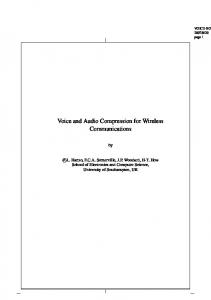
Fig. 1. The frame-level phoneme accuracy scores and the average bits per sample used for the Truncate, µ-Law and Delta methods.
Fig. 2. The frame-level phoneme accuracy scores and the average bits per sample used for the Delta method and its modified versions.
The codes are not prefixes of each other; this way decoding can be done easily by parsing the encoded stream from left to right bitwise. It is clear that the possible samples of an audio signal are usually represented unevenly, hence such a compression method could be used in this environment quite effectively. Huffman coding, however, clearly has a drawback for our purposes: it is a CPU-demanding method, which clearly cannot be applied on a wireless sensor in its basic form. Moreover, the online calculation of the codes for each packet would also require sending the list of codes, which would waste a lot of bandwidth. To overcome these problems, we had to apply a small trick: we precalculated the Huffman codes of each possible sample on a normal PC. For this the probability value (i.e. frequency) of each sample is needed, which values were calculated based on a sample recording made using the wireless sensor. This way encoding on the sensor consisted only of reading the appropriate code from a pre-calculated table for each sample value, and then these codes were put together into one packet. Note however, that during this last step the varying length of the codes had to be taken into account. Decoding on the remote side could be done by parsing the incoming packet bitwise, as in the original Huffman algorithm. The application of this variation of Huffman coding is not restricted to that of raw signals: it can be applied to practically any fixed set where the relative frequencies of elements are known. Hence we used this algorithm for every single compression method described above: e.g. for the Delta algorithm, after computing the value of ∆ for n bits, we sent its precalculated Huffman code instead of ∆. As Huffman coding is a lossless compression, it does not affect the quality of the resulting signal, just the bandwidth required to transmit it.
the testing environment, then explain the evaluation methodology applied. Finally the obtained results are presented and analysed.
IV. E XPERIMENTS AND R ESULTS Having defined the problem and the methods applied, we will now turn to the experiments section. First we will describe
– 79 –
A. Hardware In this study Crossbow Iris sensor nodes (motes) were used that have a 2.4 GHz processor with a RAM of 8K bytes and a programmable flash memory of 128K bytes. The microphone and other input peripherals are located on a piece of hardware that can be attached to it, on the so-called sensor board. Crossbow MTS300 sensor boards were used, which, besides the microphone, also contain light and temperature sensors. B. The Recordings Used Testing was performed on Hungarian broadcast news: a fiveminute-long signal recorded via the wireless sensor was used for training purposes. Firstly, for the determination of Huffman codes the relative frequency values are required, which were calculated based on this signal. Secondly, for the Delta + Multipliers and Delta + µ-Law + Multipliers methods those c multiplier values were incorporated which produced the least mean squared error values for this particular recording. For testing a longer, 23 minute-long recording was used, which contained Hungarian broadcast news from a different TV channel. This signal was used to determine the actual compression ratio of the Huffman method using the abovecalculated codes, and it was utilized to measure the performance of the low-complexity audio compression methods. C. The Evaluation Process One standard way of evaluating lossy compression methods could be to measure the difference between the input and the output signals via some kind of error function like the mean squared error. On sound signals, however, this approach has a limitation: it does not take the aspect of understandability into consideration. That is, if a compression configuration greatly modifies the input signal, but at the same time preserves its sound quality, then such an error function cannot detect it.
G. Gosztolya et al. • Low-Complexity Audio Compression Methods For Wireless Sensors
Accuracy (%)
100 97.5 95 92.5
87.5 100
Accuracy (%)
Truncate µ−Law Delta
90 4
5
6
7
8
9
97.5 95 Delta Delta + Mult. Delta + µ−Law Delta + µ−Law + Mult.
92.5 90 87.5
4
5
6
7
Average bits per sample
8
9
Fig. 3. The frame-level phoneme accuracy scores and the average bits per sample used for the methods tested, in the accuracy range 87.5 . . . 100%.
To approximate this “understandability” we turned to standard techniques of speech recognition. Apart from the fact that there are a number of already developed methods to do it in this domain, there is yet another reason: on the receiver side we probably do not want to play the transmitted signal to a human, but we would like to process it by a speech recognition system. In this case technologies from the field of speech recognition are clearly adequate to measure the quality of compression. We followed the frame-based approach [4]: we divided the speech signal into small, equal-sized parts, which – after feature extraction – were classified as one of the possible phonemes. Usually it is checked to see whether the result of this phoneme-identification matches the correct label of the corresponding frame, performed for each frame of the utterance. To do it, however, the correct labeling has to be known in advance, which requires great manual effort. As we wanted to know how the signal after compression differs from the one made without compression, we opted for the latter: the result of phoneme classification on the signal sent uncompressed was treated as the correct labeling of frames. The standard 13 MFCC coefficients along with their derivatives and the second derivatives (M F CC + ∆ + ∆∆ for short) [2] were applied as features for phoneme classification, which was performed by employing Artificial Neural Networks (ANNs) [1]. As usually several hours of hand-labeled and hand-segmented recordings are required for training, another database was used for this task [6]. This database was recorded over the phone, and not via the wireless sensors, but the recording conditions were very similar: it had a sampling frequency very close to 8861 Hz (8000 Hz) and about the same level of basic noise. The features were calculated using the HTK toolkit [7]. D. Results The phoneme-level accuracy scores of the methods tested have been plotted in figures 1 and 2. In these, the tradeoff between the compression ratio and the accuracy achieved can be readily seen: the higher the former is, the lower the latter becomes. The Truncate Method loses its accuracy
– 80 –
Method Truncate + Huffman µ-Law + Huffman µ-Law + Huffman Delta + Huffman Delta + Mult. + Huffman Delta + µ-Law + Huffman Delta + µ-Law + Mult. + Huffman Truncate + Huffman µ-Law + Huffman Delta + Huffman Delta + Mult. + Huffman Delta + Mult. + Huffman Delta + µ-Law + Huffman Delta + µ-Law + Mult. + Huffman No compression
n=9 n=8 n=9 n=9 n=9 n=9 n=9 n=8 n=6 n=8 n=7 n=8 n=6 n=7
TABLE I S OME NOTABLE PERFORMANCE SCORES OF THE
Avg. bits 6.05 6.84 7.04 6.92 6.00 6.91 6.91 5.06 5.37 6.80 4.45 5.22 5.51 6.16 10.00
Accuracy 97.74% 99.28% 99.89% 98.89% 97.16% 99.84% 99.84% 94.41% 94.76% 93.58% 93.86% 96.42% 95.52% 95.01% 100.0%
COMPRESSION METHODS .
rapidly with the decrease of bits per sent, while the µ-Law Method performs much better than this except in the 1- and 2-bit case, where the accuracy score is too low anyway. It is surprising, however, that the basic Delta Method led to worse results even at n = 8; the reason for this is probably that the n ≤ 8 bits were not enough to adequately transmit the actual ∆ values. The application of the c multipliers, however, was able to overcome this problem: the Delta + Multipliers Method performed just slightly worse than the µ-Law Method. Applying the µ-Law compression on the ∆ values also increased the efficiency of the method: the Delta + µ-Law Method proved to be the best among the Delta variations; on the other hand, using the c multiplier constants clearly reduced its performance. Concentrating on those method configurations that produced higher accuracy scores (see Figure 3), we can draw similar conclusions. The Delta + Multipliers Method performed adequately; the best ones were the µ-Law and the Delta + µ-Law methods, while the others performed quite poorly. Using Huffman coding, however, led to a surprise: most methods could be compressed only to a limited extent, with the single exception of the Truncate Method. The reason could be that the other algorithms carry out some kind of compression themselves, and sometimes this compression is based on the same principles as the Huffman coding. For example the µ-Law Method represents samples closer to the zero level more precisely (i.e. with a larger number of codes), which samples are more common than the rest; this way the other samples are combined into fewer groups, increasing their relative frequencies and making them harder to compress any further. Sadly, these compression methods did not prove to be as effective as the Huffman algorithm. It is true, however, only if we do not expect a very high accuracy score: the Truncating Method with n = 9 could only achieve 97.74%, which is significantly lower than the 99.89% score of the µLaw Method (n = 9). Due to the tradeoff between compression and accuracy, it is hard to clearly rank the compression rate of the methods tested.
SISY 2010 • 2010 IEEE 8th International Symposium on Intelligent Systems and Informatics • September 10-11, 2010, Subotica, Serbia
To make this ranking easier, we set two levels of accuracy: in the first the algorithms are expected to achieve an accuracy close to 100%, while in the second case a level around 95% is enough (see Table I). Two methods could not fulfil the first criterion: the accuracy values of 97.74% and 97.16% (Truncate and Delta + Multipliers methods, respectively) fell quite far from 100%; the remaining four methods all performed quite similarly; their 6.84 − 7.01 bits per sample (using Huffman coding) meant a 30% reduction in the required bandwidth. As for the second criterion, comparing the methods is more difficult as the minimum accuracy score is not clearly set due to the limited amount of scalability available (in practice n has to be in the range 5 . . . 9). Still, the best-performing methods are clearly the Truncate Method with n = 8 and the Delta + Multipliers Method with n = 7 and n = 8, which are just the two algorithms that failed to meet the first criterion. The accuracy scores achieved by these configurations lie between 93.86% and 96.42%, while their average required bandwidth is between 4.45 and 5.22 bits per sample, which means a 50% reduction in radio traffic. V. C ONCLUSIONS Because of the limited amount of bandwidth available for communication between wireless sensors, an important aspect that has to be considered is the compression of data sent. In our particular case wireless sensors were used for recording
– 81 –
and transmitting audio data, which led us to test algorithms for audio compression. Since wireless sensors usually have extremely weak hardware, only methods with small CPU and memory requirements could be applied. We found that even within these limitations, sufficient compression could be achieved. By using the µ-law method especially designed for audio compression, we could cut the required bandwidth by 30% with practically no information loss. On the other hand, if we allow a small information loss, the simple algorithm that discards the lower bits of samples can reduce the required bandwidth by 50% when combined with the well-known Huffman coding method. R EFERENCES [1] C. Bishop. Neural Networks for Pattern Recognition. Clarendon Press, Oxford, 1995. [2] X. Huang, A. Acero, and H.-W. Hon. Spoken Language Processing. Prentice Hall, 2001. [3] D. A. Huffman. A method for the construction of minimum-redundancy codes. Proceedings of the Institute of Radio Engineers, 40(9):1098–1101, September 1952. [4] L. Rabiner and B.-H. Juang. Fundamentals of Speech Recognition. Prentice Hall, 1993. [5] L. R. Rabiner and R. W. Schafer. Digital Processing of Speech Signals. Prentice Hall, 1978. [6] K. Vicsi, L. T´oth, A. Kocsor, and J. Csirik. MTBA – a Hungarian telephone speech database (in Hungarian). H´ırad´astechnika, LVII(8), 2002. [7] S. Young. The HMM Toolkit (HTK) (software and manual). http://htk.eng.cam.ac.uk/, 1995.