Machine Learning Applied to Airspeed Prediction During Climb

1

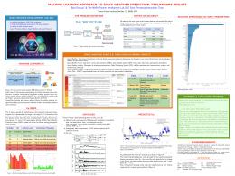
Machine Learning Applied to Airspeed Prediction During Climb R. Alligier, D. Gianazza, N. Durand ENAC, MAIAA, F-31055 Toulouse, France Univ. de Toulouse, IRIT/APO, F-31400 Toulouse, France

Abstract—In this paper, we apply Machine Learning methods to improve the aircraft climb prediction in the context of groundbased applications. Mass and speed intent are key parameters for climb prediction. As they are considered as competitive parameters by many airlines, they are currently not available to groundbased trajectory predictors. Consequently, most predictors today use reference parameters that may be quite different from the actual ones. In our most recent paper ([1]), we have demonstrated that Machine Learning techniques provide a mass estimation significantly more precise than two state-of-the-art mass estimation methods. In this paper, we apply similar techniques to the speed intent. We first build a set of examples by adjusting CAS/Mach speed profile to each climb trajectory in our database. Then, using the c) in this database, we learn a model able adjusted values (cas, c M to predict the (cas, M ) values of a new trajectory, using its past points as input. We apply this technique to actual Mode-C radar data and we consider 9 different aircraft types. When compared with the reference speed profiles provided by BADA, the reduction of the speed RMSE ranges from 36 % to 79 %, depending on the aircraft type. Using the predicted mass and speed profile, BADA is used to compute the predicted future trajectory with a 10 minute horizon. When compared with BADA used with the reference parameters, the reduction of the future altitude RMSE ranges from 45 % to 87 %.

Keywords: aircraft trajectory prediction, speed intent, BADA, Machine Learning I NTRODUCTION Trajectory prediction is a key feature to most Air Traffic Management and Control (ATM/ATC) operational concepts. The role of trajectory prediction is even more important in the future concepts and decision support tools envisioned in the European SESAR program ([2]) and its U.S. counterpart NextGen ([3]). With the implementation of a data-link between aircraft and ground-based systems, one could think that the on-board trajectory prediction could be downloaded to the groundbased system. However, for some applications the groundbased trajectory prediction is still more relevant. Some of the most recent algorithms designed to solve ATM/ATC problems do require to test a large number of alternative trajectories and it would be impractical to download them all from the aircraft. As an example of such algorithms, in [4] an iterative quasiNewton method is used to find trajectories for departing aircraft, minimizing the noise nuisance. Another example is [5] where Monte Carlo simulations are used to estimate the risk

of conflict between trajectories in a stochastic environment. Some of the automated tools currently being developped for ATM/ATC can detect and solve conflicts between trajectories (see [6] for a review). These algorithms may use Mixed Integer Programming ([7]), Genetic Algorithms ([8], [9]), Ant Colonies ([10]), or Differential Evolution or Particle Swarm Optimization ([11]) to find optimal solutions to air traffic conflicts. To be efficient, all these methods require a fast and accurate trajectory prediction, and the capability to test a large number of “what-if” trajectories. Such requirements forbid the sole use of on-board trajectory prediction, which is certainly the most accurate, but which is not directly available to ground systems. Most trajectory predictors rely on a point-mass model to describe the aircraft dynamics. The aircraft is simply modeled as a point with a mass, and the second Newton’s law is applied to relate the forces acting on the aircraft to the inertial acceleration of its center of mass. Such a model is formulated as a set of differential algebraic equations that must be integrated over a time interval in order to predict the successive aircraft positions, knowing the aircraft initial state (mass, current thrust setting, position, velocity, bank angle, etc.), atmospheric conditions (wind, temperature), and aircraft intent (thrust profile, speed profile, route). Unfortunately, the data that is currently available to groundbased systems for trajectory prediction purposes is of fairly poor quality. The speed intent and aircraft mass, being considered competitive parameters by many airline operators, are not transmitted to ground systems. The actual thrust setting of the engines (nominal, reduced, or other, depending on the throttle’s position) is unknown. Weather and Radar data are uncertain. The problem of unknown parameters such as the mass, thrust law, and target speeds, is of particular importance when predicting the aircraft climb. Figure 1 illustrates the climb prediction problem, when using a physical model of the aircraft dynamics. Some studies ([12], [13], [14]) detail the potential benefits that would be provided by additional or more accurate input data. In other works, the aircraft intent is formalized through the definition of an Aircraft Intent Description Language ([15], [16]) that could be used in air-ground data links to transmit some useful data to ground-based applications. All the necessary data required to predict aircraft trajectories might become available to ground systems someday. In the meantime, by applying Machine Learning techniques, we propose to learn

2

this set of examples, we learn a model able to predict (cas, M ) values from the past points of a new input trajectory.

Aircraft intent: Thrust setting law: ? Speed Profile: ? Physical model Aircraft state at t0 : Mass: ? (Position,Speed)

Future trajectory

Aircraft intent: Thrust setting law: max,climb Speed Profile: (casref , Mref )

max,climb (casref , Mref ) BADA files

BADA: Base of Aircraft Data

Physical model

Aircraft state at t0 : Mass: mref (Position,Speed)

mref

Future trajectory

Past points

Past points

Figure 1: The ground-based aircraft climb prediction problem.

some of the unknown parameters of the point-mass model from the data that is already available today, typically from the observed radar tracks of past and current flights. Applying Machine Learning techniques on the trajectory prediction problem is not a new idea. A decade ago, [17] has applied artificial neural network on this problem. It has also been investigated more recently using different Machine Learning techniques ([18], [19], [20]). With these approaches, the obtained model directly predicts the trajectory. It is a blackbox hiding what comes from the aircraft performances and what comes from the airline procedures, i.e. the way it is operated. In this context, the originality of our work is that we keep the physical model in the loop. The physical model describes the aircraft performances and the data-driven models describe how the aircraft is operated i.e. the mass and the speed intent. In current operation, the trajectory is predicted by using the reference mass and the reference (casref , Mref ) values from the Eurocontrol Base of Aircraft Data (BADA) (see Figure 2). These values describe the speed profile of a climbing aircraft. The aircraft climbs at constant CAS (Calibrated Airspeed) equals to cas till the transition altitude is reached, then it climbs at a constant Mach M . Although BADA associates one (cas, M ) value to each aircraft type, these values might be different among aircraft of the same type due to different cost-index for instance. In this paper, using all the information available, we want to predict a (cas, M ) value specific to the considered aircraft. Figure 3 describes the approach developed in this paper to improve trajectory prediction using Machine Learning techniques. Using these techniques allows us to build the predictive models hm , hcas and hM . In previous paper [1], we describe how the model hm predicting the mass is obtained. We demonstrated that the model hm was significantly more precise than two mass estimation methods previously compared in [21]. In the current paper, we want to predict the speed profile. Todo so, we build a set of examples by adjusting  c speed profile to each trajectory of a recorded set a cas, c M of trajectories. Then, using Machine Learning techniques on

Figure 2: Baseline method : the BADA prediction of the future aircraft climb

Aircraft intent: Thrust setting: max,climb Speed Profile: (hcas (x), hM (x)) Physical model Aircraft state at t0 : Mass: hm (x) (Position,Speed)

Predictive models h x

Future trajectory

Past points

Figure 3: This figure describes how the future trajectory is predicted by applying Machine Learning techniques. When a fresh trajectory is observed, the input variables x are computed from the observed points and the predictive models hm , hcas and hM are used to predict the mass and the speed profile. The rest of this paper is organized as follows: Section I presents some useful Machine Learning notions that help understanding the methodology applied in our work. Section II details the data used in this study. The application of Machine Learning techniques to our speed profile prediction problem is described in section III, and the results are shown and discussed in section IV, before the conclusion. I. M ACHINE L EARNING This section describes some useful Machine Learning notions and techniques. For a more detailed and comprehensive description of these techniques, one can refer to [22], [23]. As explained in the previous section, we want to predict c values of a given a variable y, here the adjusted cas c and M

3

trajectory, from a vector of explanatory variables x, which in our case is the data extracted from the past trajectory points and the weather forecast. This is typically a regression problem. Naively said, we want to learn a function h such that y = h(x) for all (x, y) drawn from the distribution (X, Y ). Actually, such a function does not exist, in general. For instance, if two ordered pairs (x, y1 ) and (x, y2 ) can be drawn with y1 6= y2 , h(x) cannot be equal to y1 and y2 at the same time. In this situation, it is hard to decide which value to give to h(x). A way to solve this issue is to use a real-valued loss function L. This function is defined by the user of function h. The value L(h(x), y) models a cost for the specific use of h when (x, y) is drawn. With this definition, the user wants a function h minimizing the expected loss R (h) defined by equation (1). The value R (h) is also called the expected risk. R(h) = E(X,Y ) [L (h(X), Y )]

(1)

However, the main issue when choosing a function h minimizing R (h) is that we do not know the joint distribution (X, Y ). We only have a set of examples of this distribution. A. Learning from examples Let us consider a set of n examples S = (xi , yi )16i6n coming from independent draws of the same joint distribution (X, Y ). We can define the empirical risk Rempirical by the equation below: 1 X L (h(x), y) . (2) Rempirical (h, S) = |S| (x,y)∈S

Assuming that the values (L(h(x), y))(x,y)∈S are independent draws from the same law with a finite mean and variance, we can apply the law of large numbers giving us that Rempirical (h, S) converges to R(h) as |S| approaches +∞. Thereby, the empirical risk is closely related to the expected risk. So, if we have to select h among a set of functions H minimizing R(h), using a set of examples S, we select h minimizing Rempirical (h, S). This principle is called the principle of empirical risk minimization. Unfortunately, choosing h minimizing Rempirical (h, S) will not always give us h minimizing R(h). Actually, it depends on the “size”1 of H and the number of examples |S| ([24], [25]). The smaller H and the larger |S| are, the more the principle of empirical risk minimization is relevant. When these conditions are not satisfied, the selected h will probably have a high R(h) despite a low Rempirical (h, S). In this case, the function h is overfitting the examples S. These general considerations above have practical consequences on the use of Machine Learning. Let us denote hS the function in H minimizing Rempirical (., S). The expected risk using hS is given by R(hS ). We use the principle of 1 The

“size” of H refers here to the complexity of the candidate models contained in H, and hence to their capability to adjust to complex data. As an example, if H is a set of polynomial functions, we can define the “size” of H as the highest degree of the functions contained in H. In classification problems, the “size” of H can be formalized as the Vapnik-Chervonenkis dimension.

empirical risk minimization. As stated above, some conditions are required for this principle to be relevant. Concerning the size of the set of examples S: the larger, the better. Concerning the size of H, there is a tradeoff: the larger H is, the smaller min R(h) is. However, the larger H is, the larger the gap h∈H

between R(hS ) and min R(h) becomes. This is often referred h∈H to as the bias-variance tradeoff. B. Accuracy Estimation In this subsection, we want to estimate the accuracy obtained using a Machine Learning algorithm A. Let us denote A[S] the prediction model found by algorithm A when minimizing Rempirical (., S)2 , considering a set of examples S. The empirical risk Rempirical (A[S], S) is not a suitable estimation of R(A[S]): the law of large numbers does not apply here because the predictor A[S] is neither fixed nor independent from the set of examples S. One way to handle this is to split the set of examples S into two independent subsets: a training set ST and another set SV that is used to estimate the expected risk of A[ST ], the model learned on the training set ST . For that purpose, one can compute the holdout validation error Errval as defined by the equation below: Errval (A, ST , SV ) = Rempirical (A[ST ], SV ).

(3)

Cross-validation is another popular method that can be used to estimate the expected risk obtained with a given learning algorithm. In a k-fold cross-validation method, the set of examples S is partitioned into k folds (Si )16i6k . Let us denote S−i = S\Si . In this method, k trainings are performed in order to obtain the k predictors A[S−i ]. The mean of the holdout validation errors is computed, giving us the cross-validation estimation below: CV (A, S) =

k X |Si | i=1

|S|

Errval (A, S−i , Si ).

(4)

This method is more computationally expensive than the holdout method but the cross-validation is more accurate than the holdout method ([26]). In our experiments, the folds were stratified. This technique is said to give more accurate estimates ([27]). The accuracy estimation has basically two purposes: first, model selection in which we select the “best” model using accuracy measurements and second, model assessment in which we estimate the accuracy of the selected model. For model selection, the set SV in Errval (A, ST , SV ) is called validation set whereas in model assessment this set is called testing set. C. Hyperparameter Tuning Some learning algorithms have hyperparameters. These hyperparameters λ are the parameters of the learning algorithm 2 Actually, depending on the nature of the minimization problem and chosen algorithm, this predictor A[S] might not be the global optimum for Rempirical (., S), especially if the underlying optimization problem is handled by local optimization methods.

4

Aλ . These parameters cannot be adjusted using the empirical risk because most of the hyperparameters are directly or indirectly related to the size of H. Thus, if the empirical risk was used, the selected hyperparameters would always be the ones associated to the largest H. These hyperparameters allow us to control the size of H in order to deal with the bias-variance tradeoff. These hyperparameters can be tuned using the holdout method on a validation set for accuracy estimation. In order to find λ minimizing the accuracy estimation, we used a grid search which consists in an exhaustive search on a predefined set of hyperparameters. The Algorithm 1 is a learning algorithm without any hyperparameters. In this algorithm, 20% of the training set is held out as a validation set. function T UNE G RID(Aλ ,grid)[T ] (TT , TV ) ← split(80%,20%) (T ) λ∗ ← argmin Errval (Aλ , TT , TV ) λ∈grid

return Aλ∗ [T ] end function Algorithm 1: Hyperparameters tuning for an algorithm Aλ and a set of examples T (training set).

of the considered point. Walong is the wind along the true air speed in the horizontal plane VaXY . All the computed quantities are summarized in Table I. quantities Hp Vg Va VaXY dair dground ∆T W Walong Wacross WZ θc CAS Mach 1/rsol 1/rair φ T a e = Va dV + g0 T −∆T dt − → − ˙ → ew = e + W .Va ∆T (weather grid) Walong (weather grid) m ˆ LS

II. DATA USED IN THIS S TUDY A. Data Pre-processing Recorded radar tracks from Paris Air Traffic Control Center are used in this study. This raw data is made of one position report every 1 to 3 seconds, over two months (July 2006, and January 2007). In addition, the wind and temperature data from Météo France are available at various isobar altitudes over the same two months. The raw Mode-C altitude3 has a precision of 100 feet. Raw trajectories are smoothed using splines. Basic trajectory data is made of the following fields: aircraft position (X,Y in a projection plane, or latitude and longitude in WGS84), ground velocity vector Vg = (Vx , Vy ), smoothed altitude (Hp , in feet above isobar 1,013.25 hPa), rate of climb or descent dHp dt . The wind W = (Wx , Wy ) and temperature T at every trajectory point are interpolated from the weather datagrid. The temperature differential ∆T is computed at each point of the trajectory. Using the position, velocity and wind data, we compute the true air speed Va . The successive velocity vectors allow us to compute the trajectory curvature at each point. The aircraft bank angle is then derived from true airspeed and the curvature of the air trajectory. Along with these quantities derived from the Mode-C radar data and the weather data, we have access to some quantities in the flight plan like the Requested Flight Level for instance. With the weather datagrid, we have also computed the temperature differential ∆T (weather grid) and the wind along Walong (weather grid) at each altitude of the grid. This is done by using the VaXY , the time, the latitude and the longitude 3 This altitude is directly derived from the air pressure measured by the aircraft. It is the height in feet above isobar 1013.25 hPa.

dHp dt

eLS m ˆ AD RFL Speed distance AO DEP ARR

description geopotential pressure altitude Ground Speed True Air Speed True Air Speed in the (X,Y) plane distance flown w.r.t. the air distance flown w.r.t. the ground temperature differential (cf. [28]) wind wind along VaXY wind across VaXY vertical wind drift angle Calibrated Air Speed Mach number curvature w.r.t. the ground curvature w.r.t. the air bank angle specific energy rate specific energy rate corrected from the wind effect temperature differential on a grid of different Hp wind along VaXY on a grid of different Hp estimated mass from past points using least square method [21] root mean square error obtained on the past points using the least square method estimated mass from past points using adaptive method [29] Requested Flight Level requested speed distance between airports aircraft operator departing airport arrival airport

Table I: This table summarizes the quantities available in our study.

B. Filtering Climb Segments Our dataset includes all flights departing from Paris-Orly (LFPO) or Paris-Charles de Gaulle Airport (LFPG). Needless to say, this approach can be replicated to other airports. The trajectories are filtered so as to keep only the climb segments. An additional 80 seconds is clipped from the beginning and end of each segment so as to remove climb/cruise or cruise/climb transitions. It is worth noticing that the trajectories have not been filtered on the speed profile but only on the rate of climb and the altitude. C. Building the Sets of Examples The climb segments are sampled every 15 seconds. From these sampled segments, we build examples containing exactly 51 points. In these examples, the first 11 points (past trajectory) are used to predict the mass and the speed profile. The remaining points (future trajectory) are used to compute the error between the predicted and actual trajectory. From one sampled climb segment we build as many examples as we can. For instance, from a sampled climb segment

5

containing 54 points, we can build 4 examples containing exactly 51 successive points. These 4 examples share the 48 points in the middle of the climb segment. Once these examples are built, we only keep the examples with the 11th point at an altitude superior to 15,000ft for the B744 aircraft type and 18,000ft for all the other aircraft types. Using this method, we have considered 9 aircraft types and we have built one set of examples for each aircraft type. Some of the chosen aircraft types are very different: the E145 is a short haul aircraft with a 18,500 kg reference mass while the B744 is a long haul aircraft with a 285,700 kg reference mass. Looking at Table II we see the size of the different sets. type A319 A320 A321 A332 B737 B744 B772 E145 F100

number of climbing segments 1863 5729 1866 1475 344 350 910 851 660

number of examples 15702 65514 21789 28629 2178 2750 8525 8310 7430

Table II: Size of the different sets. Only the climbing segments generating at least one example in our final examples set are counted here.

D. Adjusting the Speed Profile to Observed Points We want to learn the future speed profile. x is all the information we have at t0 and before. The future speed intentis y. From a set of examples (x, y), we learn a model h predicting the speed profile from x. The predicted speed profile h(x) will be hopefully equal to the actual speed intent y. However, the actual speed intent y is not available in our data, thus we do not have the set of examples (x, y), yet. We have to extract it from the observed trajectory. In BADA, the speed intent is characterized by two values, the cas and the M . The aircraft climbs at a constant CAS equals to cas till the transition altitude Hp trans (cas, M ) is reached. Then, the aircraft climbs with a constant Mach M . The parametrized speed is given by the equation below where f is a function given by [28], T is the temperature, R and κ are physical constants.

n X
2 Φ(cas, M ) = Va (cas, M, Hp i , Ti ) − Vai i=1

X

=

f (cas, Hp i , Ti ) − Vai


2

i/Hp i 6Hp,trans (cas,M )



X

+

M

p

κRTi − Vai

2

i/Hp,trans (cas,M ) 0. We have  tested different settings: c , “ref” denotes the “adj” denotes the adjusted values cas, c M baseline values given by BADA (casref , Mref ), “mean”  denotes  c the values given by the mean of the adjusted values cas, c M and “GBM” denotes the predicted values (casGBM , MGBM ). The “adj” setting result of the adjustment described in II-D. It is the lowest RMSE we can get using a CAS/Mach speed profile. According to this table, using the baseline, the RMSE is around 20 kts for all the aircraft types except for the B744, the E145 and the F100. For these two aircraft types, the RMSE is reduced by at least 41 % with the “mean” method. With this method, the RMSE reduction is less spectacular for the six other aircraft types with nearly no reduction for some aircraft types. This indicates that the reference speed parameters are in accordance with mean parameters of the observed trajectories for these aircraft types. However, even for these aircraft types, the prediction can still be improved by predicting a (cas, M ) value specific to the considered aircraft. This is what is done when a GBM model is used. When compared to the “mean” method, the GBM method reduces the RMSE by at least 21 %.

IV. R ESULTS AND D ISCUSSION All the statistics presented in this section are computed using a stratified 10-fold cross-validation embedding the hyperparameter selection. Figure 4 illustrates how the data is partitionned, denoting λ the hyperparameter vector. Our set

B. Computing the Predicted Trajectory Using Machine Learning and BADA In order to actually predict a trajectory using the BADA model and assuming a max climb thrust, one still has to specify

7

type A319 A319 A319 A319 A320 A320 A320 A320 A321 A321 A321 A321 A332 A332 A332 A332 B737 B737 B737 B737 B772 B772 B772 B772 B744 B744 B744 B744 E145 E145 E145 E145 F100 F100 F100 F100

speed ref mean GBM adj ref mean GBM adj ref mean GBM adj ref mean GBM adj ref mean GBM adj ref mean GBM adj ref mean GBM adj ref mean GBM adj ref mean GBM adj

mean 3.77 1.19 0.412 0.0259 2.34 1.1 0.57 0.0262 3.16 1.09 0.546 0.0285 -8.71 0.118 0.648 0.0233 8.56 0.739 0.391 -0.00503 -14.4 0.298 0.66 0.0429 -28.7 1.01 0.705 0.121 69.2 1.82 1.12 -0.0446 36.8 0.646 0.654 0.0178

stdev 20.7 20.4 12.5 7.85 21 21.2 12.6 7.71 22.9 23.1 13.5 7.83 17.6 16.4 11.6 7.03 17.5 16.5 12.4 6.82 16.7 14 11 7.17 21.2 20.8 14.7 10.9 31.7 29 16.2 8.26 19.5 19.4 12.7 5.78

mean abs 15.8 14.7 8.2 5 15.3 14.9 8 4.68 17.7 17.6 9.02 4.87 16.4 11.7 7.4 4.37 13.7 12.1 8.17 4.54 19.2 9.97 7.18 4.33 32.2 16.1 9.94 6.32 69.2 24.1 12.2 5.85 36.9 14 8.44 3.64

RMSE 21 20.5 12.5 7.85 21.2 21.2 12.6 7.71 23.1 23.1 13.5 7.83 19.6 16.4 11.6 7.03 19.4 16.5 12.4 6.82 22.1 14 11 7.17 35.6 20.8 14.7 10.9 76.1 29 16.2 8.26 41.6 19.4 12.7 5.78

max abs 123 119 103 102 134 129 114 124 115 112 117 94.6 115 115 103 81.7 110 109 112 93.4 83.5 91.1 83.6 78.2 76.2 90.7 71 71.1 166 93.3 81.2 65.3 168 132 91.1 71

Table IV: These statistics, in knots, are computed on the differences between the predicted speed and the observed
speed Va cas, M, Hp i , Ti − Vai for i such as ti > 0 (i.e. i > 11). a mass and a speed profile. Both are usually unknown from ground systems. In our experiment, we want to evaluate the impact of the predicted mass and the predicted speed profile on the trajectory prediction. The prediction of the mass was introduced in a previous paper [1] using a similar approach: a mass m b is adjusted on future points and a model predicting this adjusted mass m b from known variables is learned using GBM. This approach has been demonstrated more accurate than mass estimation methods introduced in [34], [21]. In the current paper, we adjust a CAS/Mach speed profile, and we learn two GBM models predicting the adjusted values cas c c. The overall process to predict the future trajectory and M is described in Figure 5. The mass and the speed profile are specified using the three predictive models hm , hcas and hM . C. Prediction of the Future Altitude The results obtained with our methods are described in Table V. The “ref” parameter is the BADA reference parameter. The “GBM” parameter for the mass is obtained by using the model hm . The line with “GBM” for the mass and “adj” for the speed cannot be used in an operational context as it

Examples set

Aircraft intent: Thrust setting: max,climb Speed Profile: (hcas (x), hM (x))

x

z}|{ |

{z

}

Physical model

c) y=(m, b cas, c M

Machine Learning Predictive models h x

Aircraft state at t0 : Mass: hm (x) (Position,Speed)

Future trajectory

Past points

Figure 5: This figure describes how the future trajectory is predicted by applying Machine Learning techniques. The examples set is used to build predictive models (hm , hcas , hM ). When a fresh trajectory is observed, the input variables x are computed from the observed points and the predictive models are used to predict the mass and the speed profile.

uses adjusted values. This line is only used for comparison purpose. All the other lines can be used in an operational context. The baseline method, referred as BADAref , is the line with “ref” for the mass and the speed. Our approach, referred as BADAGBM , is the line with “GBM” for the mass and the speed. These two setups can be used in an operational context: they use only the information available at the time the prediction is computed. When compared with the baseline BADAref , the use of the predicted mass and the reference speed profile reduce the RMSE on the altitude by at least 29 % for any aircraft type except the E145. Note that for this latter, the gap between the reference speed profile and the observed speed profile is fairly high with a RMSE of 76.1 kts while it is around 20 kts for the other aircraft types (see Table IV). If we consider the “mean” speed, the RMSE on the altitude is noticeably reduced only for the E145 and the F100. This was expected because these two aircraft types have the largest RMSE on the speed when using the “ref” parameter. Using the predicted speed profile, we consider the BADAGBM . If we compare this latter to the BADAref setup, the RMSE on the altitude is reduced by at least 45 % for all the aircraft types, including the E145. This reduction reaches 87 % for the B772.

A319

A320

3000

2000

2000

2000

1000

1000

0

0

0

−1000

−1000

−2000

−2000

−2000 A332

(H(ppred) − H(pobs))(t) [ft]

A321

B737

4000

3000

8000

2000

6000

1000 2000

method

4000

0

BADAGBM BADAref

2000

−1000

0

B744

0

−2000 B772

E145

F100

4000 4000

2000 2000

2000

0 0

0

−2000

−2000 0

150

300

450

600

0

150

300

450

600

0

150

300

450

600

Figure 6: This figure portrays the error on the altitude obtained by BADAref and BADAGBM for nine different aircraft types. Each time step, a boxplot shows the 5 %, 25 %, 50 %, 75 % and 95 % quantiles. The whiskers (resp. box) of the boxplot contains 90 % (resp. 50 %) of the data.

8

t [s]

9

However, the reduction obtained on the altitude by using the predicted speed profile is large only for the E145 and the F100. The impact of the speed error reduction is hidden by other sources of error. Firstly, the weather model and the BADA model are not perfect. Secondly, we have assumed a max climb thrust setting which might not be a relevant assumption for all the climb trajectories.  Thirdly,  the mass used is a predicted c values were perfectly predicted, mass. Even if the cas, c M the trajectory prediction will not be perfect. The error made in this perfect case can be read at the line with “GBM” for the mass and “adj” for the speed. Thus, even with an RMSE around 8 kts on the speed profile, the RMSE on the altitude is reduced but not greatly reduced. type A319 A319 A319 A319 A319 A320 A320 A320 A320 A320 A321 A321 A321 A321 A321 A332 A332 A332 A332 A332 B737 B737 B737 B737 B737 B744 B744 B744 B744 B744 B772 B772 B772 B772 B772 E145 E145 E145 E145 E145 F100 F100 F100 F100 F100

mass ref GBM GBM GBM GBM ref GBM GBM GBM GBM ref GBM GBM GBM GBM ref GBM GBM GBM GBM ref GBM GBM GBM GBM ref GBM GBM GBM GBM ref GBM GBM GBM GBM ref GBM GBM GBM GBM ref GBM GBM GBM GBM

speed ref ref mean GBM adj ref ref mean GBM adj ref ref mean GBM adj ref ref mean GBM adj ref ref mean GBM adj ref ref mean GBM adj ref ref mean GBM adj ref ref mean GBM adj ref ref mean GBM adj

mean 274 237 47.1 42.1 19.6 290 187 45.3 23.5 -0.895 863 33.1 37 22.1 -15.8 2622 -107 66 70.4 40.7 606 -40.8 -51.7 -52 -86.6 5558 12.4 100 142 103 3728 -80.2 99.5 112 65.7 1623 1667 548 190 68.7 556 642 193 102 43.3

stdev 1472 772 767 725 607 1420 715 718 681 523 1683 783 782 774 584 1820 673 664 651 572 1750 796 796 804 814 1646 844 842 778 748 1413 534 502 500 453 1801 2064 2115 1314 750 1879 1229 1209 1022 732

mean abs 1176 605 575 532 452 1165 553 534 490 389 1588 571 570 554 421 2783 479 469 460 393 1619 616 617 629 616 5580 649 646 586 547 3750 425 379 385 334 1909 2032 1741 1010 562 1616 1166 993 793 543

rmse 1497 808 769 726 608 1449 739 719 681 523 1891 784 783 774 584 3192 682 667 654 574 1852 797 797 805 818 5797 844 848 790 755 3987 540 512 512 458 2425 2653 2185 1327 753 1959 1387 1225 1027 734

time step. The whiskers (resp. box) of the boxplot contains 90 % (resp. 50 %) of the data.

C ONCLUSION To conclude, let us summarize our approach and findings, before giving a few perspectives on future works. In this article we have described a way to predict the future speed profile. Using Machine Learning and a set of examples, we have built models predicting the values (cas, M ) of a CAS/Mach speed profile. Using real Mode-C radar, this approach has been tested on the 9 different aircraft types. In order to evaluate the accuracy of the Machine Learning method, a cross-validation is used. When compared to the reference speed profiles provided by BADA, the RMSE on the speed is max abs reduced by at least by 36 % using GBM, a Machine Learning 5315 method. Concerning the E145, this RMSE is reduced by 79 %. 5350 In order to predict the future trajectory, this approach is used 5478 5529 in conjunction with a similar approach described in [1]. This 5720 latter is used to predict the mass. Then using the predicted 5753 mass and speed profile, the BADA physical model is used 6815 to compute the predicted future trajectory with a 10 minutes 6707 7193 horizon. The RMSE on the future altitude is reduced by at 6202 least 45 %. This reduction reaches 87 % for the B772. 6154 From an operational point of view, the resulting improve4627 ment in the climb prediction accuracy would certainly benefit 4642 4418 air traffic controllers, especially in the vertical separation task 5569 as shown in [34]. Furthermore, even if it was not computed 6769 in our study, the proposed method probably reduces the along 5217 track error and the Top Of Climb prediction error. 4997 4934 We only have considered a CAS/Mach speed profile. How4795 ever, as said before, the climbing trajectories in our data does 4157 not always follow a CAS/Mach speed profile. In order to 3672 improve the trajectory prediction, we might consider other 3667 climb procedures. For future work, we might consider a 3645 4216 procedure in which the aircraft climbs at a constant CAS cas1 10183 till the altitude H p cas , then accelerates/decelerates till the CAS 3495 reaches cas and finally follows a (cas2 , M ) CAS/Mach speed 2 3372 profile. However, in order to use this, we would 3342
have to adapt 3656 our method to predict cas1 , Hp cas , cas2 , M . 7145 3513 3647 3446 3316 7428 8280 7289 5378 5858 6539 4940 5425 4490 4587

Table V: These statistics, in feet, are computed on the differences between the predicted altitude and the observed altitude   (pred) (obs) Hp − Hp at the time t = 600 s. Figure 6 portrays the error on the altitude at different time horizons. More specifically, boxplots are presented at each

R EFERENCES [1] R. Alligier, D. Gianazza, and N. Durand. Machine learning and mass estimation methods for ground-based aircraft climb prediction. Intelligent Transportation Systems, IEEE Transactions on, submitted. [2] SESAR Consortium. Milestone Deliverable D3: The ATM Target Concept. Technical report, 2007. [3] H. Swenson, R. Barhydt, and M. Landis. Next Generation Air Transportation System (NGATS) Air Traffic Management (ATM)-Airspace Project. Technical report, National Aeronautics and Space Administration, 2006. [4] X. Prats, V. Puig, J. Quevedo, and F. Nejjari. Multi-objective optimisation for aircraft departure trajectories minimising noise annoyance. Transportation Research Part C, 18(6):975–989, 2010. [5] G. Chaloulos, E. Crück, and J. Lygeros. A simulation based study of subliminal control for air traffic management. Transportation Research Part C, 18(6):963–974, 2010. [6] James K Kuchar and Lee C Yang. A review of conflict detection and resolution modeling methods. Intelligent Transportation Systems, IEEE Transactions on, 1(4):179–189, 2000. [7] Lucia Pallottino, Eric M Feron, and Antonio Bicchi. Conflict resolution problems for air traffic management systems solved with mixed integer programming. Intelligent Transportation Systems, IEEE Transactions on, 3(1):3–11, 2002.

10

[8] J. M. Alliot, Hervé Gruber, and Marc Schoenauer. Genetic algorithms for solving ATC conflicts. In Proceedings of the Ninth Conference on Artificial Intelligence Application. IEEE, 1992. [9] N. Durand, J.M. Alliot, and J. Noailles. Automatic aircraft conflict resolution using genetic algorithms. In Proceedings of the Symposium on Applied Computing, Philadelphia. ACM, 1996. [10] Nicolas Durand and Jean-Marc Alliot. Ant colony optimization for air traffic conflict resolution. In 8th USA/Europe Air Traffic Management Research and Developpment Seminar, 2009. [11] C. Vanaret, D. Gianazza, N. Durand, and J.B. Gotteland. Benchmarking conflict resolution algorithms. In International Conference on Research in Air Transportation (ICRAT), Berkeley, California, 22/05/12-25/05/12, page (on line), http://www.icrat.org, may 2012. ICRAT. [12] Study of the acquisition of data from aircraft operators to aid trajectory prediction calculation. Technical report, EUROCONTROL Experimental Center, 1998. [13] ADAPT2. aircraft data aiming at predicting the trajectory. data analysis report. Technical report, EUROCONTROL Experimental Center, 2009. [14] R. A. Coppenbarger. Climb trajectory prediction enhancement using airline flight-planning information. In AIAA Guidance, Navigation, and Control Conference, 1999. [15] J. Lopez-Leones, M.A. Vilaplana, E. Gallo, F.A. Navarro, and C. Querejeta. The aircraft intent description language: A key enabler for airground synchronization in trajectory-based operations. In Proceedings of the 26th IEEE/AIAA Digital Avionics Systems Conference. DASC, 2007. [16] J. Lopes-Leonés. The Aircraft Intent Description Language. PhD thesis, University of Glasgow, 2007. [17] Y. Le Fablec. Prévision de trajectoires d’avions par réseaux de neurones. PhD thesis, Thèse doctorat informatique de l’INPT, 1999. [18] K. Tastambekov, S. Puechmorel, D. Delahaye, and C. Rabut. Aircraft trajectory forecasting using local functional regression in sobolev space. Transportation Research Part C: Emerging Technologies, 39(0):1 – 22, 2014. [19] M. Ghasemi Hamed. Méthodes non-paramétriques pour la prévision d’intervalles avec haut niveau de confiance: application à la prévision de trajectoires d’avions. PhD thesis, Thèse doctorat informatique de l’INPT, 2014. [20] Marko Hrastovec and Franc Solina. Machine learning model for aircraft performances. In Digital Avionics Systems Conference (DASC), 2014 IEEE/AIAA 33rd, pages 8C4–1. IEEE, 2014. [21] R. Alligier, D. Gianazza, and N. Durand. Ground-based estimation of aircraft mass, adaptive vs. least squares method. In 10th USA/Europe Air Traffic Management Research and Developpment Seminar, 2013. [22] T. Hastie, R. Tibshirani, and J. H. Friedman. The Elements of Statistical Learning. Springer Series in Statistics. Springer New York Inc., New York, NY, USA, 2001. [23] C. M Bishop. Pattern recognition and machine learning, volume 1. springer New York, 2006. [24] Vladimir N. Vapnik and Alexey Ya. Chervonenkis. The necessary and sufficient conditions for consistency of the method of empirical risk minimization. Pattern Recogn. Image Anal., 1(3):284–305, 1991. [25] Vladimir N. Vapnik. The nature of statistical learning theory. SpringerVerlag New York, Inc., New York, NY, USA, 1995. [26] Avrim Blum, Adam Kalai, and John Langford. Beating the hold-out: Bounds for k-fold and progressive cross-validation. In Proceedings of the twelfth annual conference on Computational learning theory, pages 203–208. ACM, 1999. [27] R. Kohavi. A study of cross-validation and bootstrap for accuracy estimation and model selection. pages 1137–1143. Morgan Kaufmann, 1995. [28] A. Nuic. User manual for base of aircarft data (bada) rev.3.9. Technical report, EUROCONTROL, 2011. [29] C. Schultz, D. Thipphavong, and H. Erzberger. Adaptive trajectory prediction algorithm for climbing flights. In AIAA Guidance, Navigation, and Control (GNC) Conference, August 2012. [30] Jerome H. Friedman. Stochastic gradient boosting. Computational Statistics Data Analysis, 38(4):367 – 378, 2002. [31] J. H. Friedman. Greedy function approximation: A gradient boosting machine. Annals of Statistics, 29:1189–1232, 2000. [32] L. Breiman, J. H. Friedman, R. A. Olshen, and C. J. Stone. Classification and Regression Trees. Statistics/Probability Series. Wadsworth Publishing Company, Belmont, California, U.S.A., 1984. [33] G. Ridgeway. Generalized boosted models: A guide to the gbm package. Update, 1:1, 2007.

[34] C. Schultz, D. Thipphavong, and H. Erzberger. Adaptive trajectory prediction algorithm for climbing flights. In AIAA Guidance, Navigation, and Control (GNC) Conference, August 2012.

B IOGRAPHIES Richard Alligier received his Ph.D. (2014) degree in Computer Science from the "Institut National Polytechnique de Toulouse" (INPT), his engineer’s degrees (IEEAC, 2010) from the french university of civil aviation (ENAC) and his M.Sc. (2010) in computer science from the University of Toulouse. He is currently assistant professor at the ENAC in Toulouse, France. David Gianazza received his two engineer degrees (1986, 1996) from the french university of civil aviation (ENAC) and his M.Sc. (1996) and Ph.D. (2004) in Computer Science from the "Institut National Polytechnique de Toulouse" (INPT). He has held various positions in the french civil aviation administration, successively as an engineer in ATC operations, technical manager, and researcher. He is currently associate professor at the ENAC, Toulouse. Nicolas Durand graduated from the Ecole polytechnique de Paris in 1990 and the Ecole Nationale de l’Aviation Civile (ENAC) in 1992. He has been a design engineer at the Centre d’Etudes de la Navigation Aérienne (then DSNA/DTI R&D) since 1992, holds a Ph.D. in Computer Science (1996) and got his HDR (french equivalent of tenure) in 2004. He is currently professor at the ENAC/MAIAA lab.