Machine Learning in Production Systems Design Using ... - CiteSeerX

International Journal of Computational Intelligence Volume 4 Number 1

Machine Learning in Production Systems Design Using Genetic Algorithms Abu Qudeiri Jaber, Yamamoto Hidehiko and Rizauddin Ramli arbitrary kinds of constraints and objectives; all such things can be handled as weighted components of the fitness function, making it easy to adapt the GA scheduler to the particular requirements of a very wide range of possible overall objectives. GA is one of the wide applicability of knowledge-learn problem-solving tools that can provide an approach [1], [2]. While the great advantage of GA is the fact that they find a solution through evolution, this is also the biggest disadvantage. Evolution is inductive; in nature life does not evolve towards a good solution but it evolves away from bad circumstances. This can cause a species to evolve into an evolutionary dead end. In order to reduce the effect of this disadvantage a learning tool is add to the GA to decide whether is effective to continue with the generated population or the current population, this learning tool is called hereafter as keeping efficient population (KEP).

Abstract—To create a solution for a specific problem in machine learning, the solution is constructed from the data or by use a search method. Genetic algorithms are a model of machine learning that can be used to find nearest optimal solution. While the great advantage of genetic algorithms is the fact that they find a solution through evolution, this is also the biggest disadvantage. Evolution is inductive, in nature life does not evolve towards a good solution but it evolves away from bad circumstances. This can cause a species to evolve into an evolutionary dead end. In order to reduce the effect of this disadvantage we propose a new a learning tool (criteria) which can be included into the genetic algorithms generations to compare the previous population and the current population and then decide whether is effective to continue with the previous population or the current population, the proposed learning tool is called as Keeping Efficient Population (KEP). We applied a GA based on KEP to the production line layout problem, as a result KEP keep the evaluation direction increases and stops any deviation in the evaluation.

Keywords—Genetic algorithms, Layout problem, Machine learning, Production system.

T

II. GENETIC ALGORITHMS The GA paradigm has been proposed to solve a wide range of problems [2][3][4]. GA has been successfully applied to optimization problems in diverse fields and it is differs from other search techniques which depend on natural genetic evaluation process. GA starts with an initial set of solutions selected randomly called population. A suitable encoding for each solution in the population is used to allow computation of the fitness. The solution set in the population, called as chromosome or individual, represents a solution to the optimization problem. Each individual contains a number of genes. The individuals in the initial population are evaluated to measure its fitness. To create the next population, new individuals are formed by either merging two individuals from the current population using a crossover operator or modifying an individual solution using mutation operator. Based on the individuals’ fitness, the individuals to be included in the next population are then probabilistically selected from the set of individuals in current population. The iteration, called a generation is continued until the fitness reaches its maximum value, with the hope that strong parent will create a fitter generation of the children. The best overall solution becomes the candidate solution to the problem. To create the next generation GA based on three operations: Selection, crossover and mutation.

I. INTRODUCTION

O create a solution to a specific problem in machine learning, the solution is constructed from the data or by use a search method to find nearest optimal solution. Genetic algorithm (GA) is stochastic search which is often used in machine learning application. An effective GA representation and meaningful fitness evaluation is the keys of the success in GA applications. The effectiveness of GA comes from their simplicity as robust search algorithm as well as from their power to discover good solutions rapidly for difficult high-dimensional problems. GA is useful and efficient in the following cases: ① When the search space is large, complex or poorly understood. ② When the domain knowledge is scarce or expert knowledge is difficult to encode to narrow the search space. ③ If no mathematical analysis is available. ④ When the traditional search methods fail. The advantage of the GA approach is that it can handle Manuscript received November 30, 2006. A. J. Author is with Intelligent Manufacturing Systems Laboratory, Gifu University. 1-1 Yanagido, Gifu Shi, 501-1193, Japan. (e-mail: [email protected]) Y. H. Author, is with Intelligent Manufacturing Systems Laboratory, Gifu University. 1-1 Yanagido, Gifu Shi, 501-1193, Japan. (corresponding author, phone: 81-293-2550; fax:81-293-2550;.e-mail: [email protected]). R. R. Author is with Intelligent Manufacturing Systems Laboratory, Gifu University. 1-1 Yanagido, Gifu Shi, 501-1193, Japan. (e-mail: [email protected])

A. Basic Genetic Algorithm The outline of the basic GA is described below. 1. [Start] Generate random population of n individuals (suitable solutions for the problem).

72


2. 3.

4.

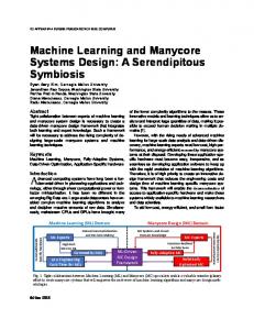
1. The size of the population of solutions, which will determine the diversity of solutions that the algorithm evaluates, and therefore the chance of an optimal solution being found [5]. 2. The ability of the algorithm to maintain diversity in the population [6]. The flow chart of GA operations is shown in figure 1.

[Fitness] Evaluate the fitness f(x) of each individual x in the population. [New population] Create a new population by repeating following steps until the new population is complete. ● [Selection] Select two parent individuals from a population according to their fitness (the better fitness, the bigger chance to be selected) ● [Crossover] With a crossover probability cross over the parents to form a new offspring (children). If no crossover was performed, offspring is an exact copy of parents. ● [Mutation] With a mutation probability mutate new offspring at each locus (position in individual). ● [Accepting] Place new offspring in a new population [Replace] Use new generated population for a further run of algorithm

B. Using Genetic Algorithms as the Search Procedure Genetic algorithms typically maintain a constant-sized population of individuals which represent samples of the space to be searched. Each individual is evaluated on the basis of its overall fitness with respect to the given application domain. New individuals (samples of the search space) are produced by selecting high performing individuals to produce "offspring" which retain many of the features of their "parents". The result is an evolving population that has improved fitness with respect to the given goal. The solution process will generate a large amount of information that can be used to carry out some form of learning.

Gen. 0 Create initial random Evaluate fitness of each individual in population yes

Is the fitness become constant? No I=0 Gen. =Gen.+1 Print the result

yes

Print the result End

I=M? No

Select Genetic Operation Probabilistically Pc Select two individual Based on fitness

Pm Select two individual Based on fitness

I=I+1

Select two gene places randomly and exchange it

Perform Crossover

Copy into new Population

Insert two offspring into new population

I=I+1 Fig. 1 GA operations flow chart

5.

[Test] If the end condition is satisfied, stop, and return the best solution in current population 6. [Loop] Go to step 2 The success of a genetic algorithm depends largely on two factors:

C. Keeping efficient population In the conventional GA, the set of possible solutions from one population are taken and are used to construct a new population. This is motivated by a hope that the new population will be fitter than the old one. Evolution evolves away from

73


bad circumstances. This can cause a species to evolve into an evolutionary dead end. This research aims to keep the evaluation direction increase and stop any deviation in the evaluation. In order to achieve this, we proposed a KEP. KEP is anew learning tool which can be included into the genetic algorithms operations to keep the efficient population. KEP is added to the GA to decide whether is effective to continue with the previous population or the current population. The main difference between the conventional GA and GA with KEP is that the conventional GA are used the current population for learning to produce the next generation. In contract, GA with KEP is first compare the current population with the previous population, and then decides whether is effective to continue with the previous population or the current population. By this way KEP is stopped any deviation in the evaluation.

Where AF The required area needed to create the new FTL layout. AP The available plant area. Dk The last machine drop point. IV. SEARCH A FTL LAYOUT USING GA In order to find an efficient layout of the FTL components through the available plant area, a GA is included into the OOLM. The OOLM is conducted using the following algorithm. Before describing the algorithm, the notations and terms used in algorithm are defined. A. Notations

Number of machines in the FTL. Buffer allocation between machines i and i+1. Side length of each cell. Sl c Li Overall machine length. Wi Overall machine width. L Overall plant length. W Overall plant width. l Side length of the buffer space. Blocked-cells(i) Number of cells included in blocked area i. Machine-cells(i) Number of cells included in machine layout i. Blocked-areas Number of blocked areas throughout the extended area. Cell through the plant area that represents C start the FTL start point. Cend Cell through the plant area that represents the FTL end point. Location of cell j in a machine i cell map c ij → p K Bi

III. PRODUCTION LINE LAYOUT PROBLEM One of the problems encountered of the design and implementation of a flexible transfer line (FTL) is the layout of the FTL in the restricted area. The layout of the FTL has an important impact on production cost. The efficient layout design of the FTL can reduce the cost of material handling by at least 10-30%. Depending on the production system, between 15% - 70% of the total production cost can be attributed to material handling [7]. Thus, the FTL layout is important to reduce production cost. The FTL layout problem is identified as a NP-complete problem [8], and many heuristic approaches have been developed to solve this problem for near optimum solution [7] – [19]. However, despite the many existing methodologies regarding the FTL layout problem, almost all approaches studing this problem neglect important operational details such as the buffer size between the machines and restricted areas in the plant area.In this paper operational details including the movement of the products between machines are considered, in addition to the restricted areas in the site. In order to find FTL layout including machines and a material handling path between each pair of machines, an efficient FTL layout design procedure called a One by One Layout Method (OOLM) in conjunction with GA is proposed. The OOLM generates an efficient solution for a set of irregularly shaped machines through a restricted plant area. The OOLM is not limited to a single static environment, but is highly flexible, within the plant structure. A CAD system is linked to the proposed OOLM to draw the FTL layout. The problem can be described mathematically as follows: Given: ● A set of K irregular-shaped machines and their dimensions; ● Spaces and machine allocation limitations; ● The plant restrictions, such as plant columns, walls, and any other restrictions in the plant area; ● The buffer size vector [B1, B2,…, BK-1]. Determine: FTL layout design. So as to minimize AF . With the following condition AF ≤ AP and Dk is located at or is close to the FTL end point.

cbki

cp i cd i

relative to the machine pick point. Location of cell k in blocked area i. Cell location of the machine i pick point through the plant area. Cell location of the machine i drop point through the plant area.

B. Definitions In order to find an efficient layout of the FTL components through the available plant area, a GA is included into the OOLM. The OOLM is conducted using the following algorithm. Before describing the algorithm, the notations and terms used in algorithm are defined. [Definition 1] Machine pick point,Pi: The machine pick point is the point where the parts input into machine i. [Definition 2] Machine drop point,Di: The machine drop point is the point where the parts leave machine i. i [Definition 3] Machine cells group, M cells − group : The machine

cells group is the set of cells that has been mapped to machine i relative to the Pi cell. [Definition 4] Buffer-cell ratio, Bm-c: The buffer–cell ratio is

74


The possible locations of the drop point are cells 1, 2, 3 and 4 in Figure 3.

the smallest integer number greater than or equal to the division of the buffer side length to the cell length; Bm-c can be calculated by using equation 2. l Bm − c = c (1) Sl [Definition 5] FTL Components: FTL components include the machines and buffer spaces. i [Definition 6] FTL Component location, COM location : The component location is the location of the next component with respect to the current component in the FTL. The component can be located in one of four locations with respect to the current component (up, down, right or left). [Definition 7] Extended plant area, Aplant-ext : The extended plant area is the area of the rectangle that passes through some of the plant outside wall and includes all plant facilities and sub walls. [Definition 8] Blocked area: The blocked area is the area in the plant that has been restricted by some robstacles such as plant columns, partitions, and sub areas used by built stations, etc. The blocked areas are not usable for allocation of machines or buffers. In addition to the blocked areas in the plant area, the areas in the extended area that are not included within the plant area are assumed to be blocked areas. i [Definition 9] Block area cells group, BAcells − group : The

2

1

4

Fig. 3 Possible locations of machine drop point i [Definition 12] Buffer space possible locations, BS drop ( j) :

The buffer space i possible locations are the locations of the buffer space i with respect to the location of the component i-1. To describe the buffer space possible locations, the following example is introduced. Example : Consider machine i in Figure 2 and assume that the buffer size next to this machine is 5. The possible locations of all buffers are shown in Figure 4 below. The possible locations of the first buffer space are the cells coded by the number 1, and the possible locations of the second buffer space are the cells that are coded by te number 2, and so on.

blocked area cells group is the set of cells that have been mapped to the blocked area i. i [Definition 10] Machine cells map, M map : The machine cells

5

P

map is the set of cells that have been mapped to the machine layout. The location of each cell in the machine map is defined relative to the machine pick point. [Definition 11] Machine drop point possible locations, i Cdrop ( j ) : The machine drop point possible locations are the

5 4

D 5

4 5

5 4 3 2 1 2 3 4 5

5 4 3 2 3 4 5

5 4 3 4 5

5 4 5

5

Fig. 4 The possible locations of the buffers.

[Definition 13] FTL area, AF: The FTL area is the area used by the FTL components. [Definition 14] Plant area, AP : The plant area is the available factory area.

locations of the machine drop points with respect to a given machine pick point. As follows [19], the machine can be located at 0, 90, 180 or 270, thus 1 ≤ j ≤ 4 . To describe the machine drop point’s possible locations, the following example is introduced. Example: Based on machine i with its pick and drop points as shown in Figure 2. Pi

p

3

C. OOLM Algorithm Step 1: Define the matrix that represents the extended plant layout area as follows : Following [18], the plant in this study is defined as uniform squares connected together and denoted in this paper as cells as shown in Figure 2. The restricted areas (obstacles) including the plant columns and any other obstacles are indicated on the plant layout. The start point and the end point of the FTL locations are given and are represented on the plant layout. The plant model can be defined by using the following steps. 1. Draw the smallest rectangle that passes through the outside walls to include all plant facilities and sub walls. The area covered by this rectangle is denoted in this paper as the extended plant area. 2. Divide the extended plant area into uniform cells that are equal to each other and connected to each other. 3. Define a matrix that represents the extended plant layout area as shown in equation 1,

Di

Fig. 2 Machine model

If the machine pick point is located at cell (I,J) then the location of the drop point possible locations are as follows: i k (I, J + 3) if M map ∉ BAcells − groups ∀ k = 1 K blocked - areas , i k (I, J - 3) if M map ∉ BAcells − groups ∀ k = 1 K blocked - areas , i k (I + 1, J) if M map ∉ BAcells − groups ∀ k = 1 K blocked - areas , i k (I - 1,J) if M map ∉ BAcells − groups ∀ k = 1K blocked - areas

75


C (1,2) ⎡ C (1,1) ⎢ C (2,1) C (2,2) ⎢ ⎢ M M ⎢ C (i ,2) ⎢ C (i ,1) ⎢ M M ⎢ ⎢C (m − 1,1) C (m − 1,2) ⎢ C (m,1) C (m,2) ⎣

L L M L M

C (1, j ) L M C (i , j ) M

L L M L M

C (1,n − 1) C (2,n − 1) M C (i ,n − 1) M

L C (m − 1, j ) L C (m − 1,n − 1) L C (m , j ) L C (m ,n − 1)

C (1,n ) C (2,n ) M

⎤ ⎥ ⎥ ⎥ ⎥ C (i ,n ) ⎥ ⎥ M ⎥ C (m − 1,n )⎥ C (m ,n ) ⎥⎦

(2)

i=1

(3)

AF - AT ≥ 0

(4)

V. GENETIC ALGORITHMS OPERATIONS FOR PRODUCTION LINE LAYOUT PROBLEM The GA operations for the production line layout problem are described in sections V.A ~ V.D. A. Encoding One of the important jobs to use GA is how to express a chromosome. One of the main difficulties in encoding this problem is that each pair of components in the FTL is located relative to each other, which it means that each component’s location should be specifically identified in the individual. This research adopts each component’s location in the FTL as the gene, each machine in the FTL represented by two genes one for the machine pick point location and the other for the machine drop point location. The other component’s locations are represented by one gene for each. The conventional GA operations are generally based on an individual with a similar gene size. In the case that we are studying here, namely FTL layout, it is difficult to use a similar gene size in individuals. This is because the number of possible component locations is not equal for all components. The number of possible location for next component is decided according to the state of locations up, down, left and right of the current component. For example if component i is located at cell (I , J), then the number of possible locations, NPL, of component i+1 is as follows:

Step 4: Read the FTL end point. Set Cend = c (i, j ), i ∈ {1,K , m}, j ∈ {1,K , n}

k and c(i, j ) ∉ BAcells − groups ∀ k = 1 K blocked - areas .

i Step 5: Define the cells map for all machines, M cells − group

relative to the Pi cell. i i i i Set M cells − group = c1→ p ,c2→ p ,K,cmachine− cells(i)→ p ∀ i = 1, K, K .

}

Step 6: Define the drop cell for machine i, relative to the Pi cell. Step 7: Define all blocked areas cells group through the i i extended plant area, BAcells − group . Set BAcells− group ∈ Aplant- ext ,

{

i =1

Then: draw the FTL, Else: read new buffer size vector [B1, B2,…, BK-1].

k and c(i, j ) ∉ BAcells − groups ∀ k = 1 K blocked - areas .

i i i i BAcells − group = cb1 , cb2 ,K , cbBlocked − cells( i )

K −1

Step 19: Carry out the following rule. If: the evaluate equation 4 is satisfied,

where C(i,j) represents the cell located in row i and column j. Step2:Set C(k) = C(i, j) ∀k = 1,2,K,(m×n),i =1,2,K,mand j = 1,2,K,n. Step 3: Read the FTL start point. Set Cstart = c(i, j ), i ∈{1,K, m}, j ∈{1,K, n}

{

∑ (B i × l 2 )

K

A T = ∑ (L i × W i ) +

}

∀i = 1,2,K,Blocked− area . Step 8: Set the first machine pick point at the FTL start point. Set P1 = C start .

Step 9: Find all possible locations of the first machine drop points, cd 1 , as described in definition 11. Step 10: Randomly select one of the possible locations of the machine drop points. Step 11: Find all possible locations of the first buffer space with respect to the machine drop point as described in definition 12. Step 12: Randomly select one of the possible locations of the first buffer space. Step 13: Find all possible locations of the next buffer space with respect to the current buffer space location and randomly select one of these locations. Step 14: Repeat step 13 to find one location for each space of buffer size. Step 15: Find all possible locations of the next machine pick points, cp i , with respect to the last buffer space and randomly select one of these locations. Step 16: Repeat steps 13 - 15 to find one of the possible locations of all machines and spaces of all buffers. Step 17: Apply the GA operations to find the best locations for all of the FTL components. Step 18: Calculate the FTL area by using equation 3.

⎧0 if the costrains 1, 2, 3, and 4 are satisfied ⎫ ⎪1 if three costrains from costrains 1, 2, 3, and 4 are satisfied ⎪ ⎪⎪ ⎪⎪ NPL = ⎨2 if two costrains from costrains 1, 2, 3, and 4 are satisfied ⎬ ⎪3 if one costrains from costrains 1, 2, 3, and 4 is satisfied ⎪ ⎪ ⎪ ⎪⎩4 if the costrains 1, 2, 3, and 4 are not satisfied ⎪⎭

(5)

Constrain 1: i (I, J + 1) ∈ { cb1i ,cb2i ,K ,cbBlocked − cells( i ) } ∀i = 1,2 ,K , Blocked − area

Constrain 2: i (I, J − 1) ∈ { cb1i ,cb 2i ,K ,cb Blocked

− cells ( i )

} ∀ i = 1 ,2 ,K , Blocked − area

− cells ( i )

}

∀ i = 1 ,2 ,K , Blocked − area

− cells ( i )

}

∀ i = 1 ,2 ,K , Blocked − area

Constrain 3: i (I + 1, J) ∈ { cb 1i ,cb 2i ,K , cb Blocked

Constrain 4: i (I - 1, J) ∈ { cb 1i ,cb 2i ,K , cb Blocked

In this research, we propose a new individual encode method to express each individual. The new encode method is called a one to one encoding method (OOEM). The following paragraph describes how to use OOEM to encode the components in the FTL. The first element in the individual represents the location of the drop point of the first machine in the FTL. The location of the first machine drop point can be

76


check the cell location leaving that cell location in the second parent. If the cell location is empty, choose the cell of the second parent otherwise choose the cell of the first parent. For example, consider the two parents as shown in Fig. 6. If the first individual is chosen as the template, child 1 can be generated using the following steps: Step 1: Select cell U (the first cell location in the iduvidual) as the first cell location of child 1. Step 2: Find the edges after gene 1 in both parents with respect to the first cell location of child 1 : (first cell location, U), read as the cell up to the first cell location and (first cell location, L), read as the cell left to the first cell location, find the cell state of these two edges. If the cell located left to the first cell location is empty (neither restricted nor used by another components) then it will be chosen as the second gene for the child 1, otherwise, the cell up to the first cell location will be chosen as the second gene for the child 1. Assuming that the cell up to the first cell location is empty, we select U as the next gene of child 1.

determined with respect to the location of the first machine pick point as described in definition 11. Elements 2, 3, …, GB1+1 in the individual represent the location of the spaces of the first buffer. The location of the first buffer space is determined with respect to the location of machine drop point and the location of next buffer space is determined with respect to the current buffer space location and so on. Figure 5 shows the encoding using the OOEM. The number of genes in each individual, T, is calculated using Eq. (6). K −1 ⎞ ⎛ T = ⎜ 2 K − 1 + ∑Bi ⎟ i =1 ⎠ ⎝

(6)

The number of items in the individuals is not limited, which means that any production line with any number of machines and any buffer size between each pair of machines can be dealt with M1

B1

…

Mi

…

Bi

BK-1

Pick S1 S2 …

[G1

G2 G3 … GB1+1

GB1+2

MK Drop

… S k

GB1+3 … Gi …

GT-1 GT]

Fig. 5 OOEM Encoding method

B. Initial population The initial population is randomly selected. The initial population contains (N) number of individuals. Each individual expresses a buffer size as shown in Figure 6. The location of components should be specifically identified in the individual because each pair of components in the FTL is located relative to each other. The initial population is determined as follows: Set individual (i) = [G1 G2 … GT-1 GT] ∀ i = 1, 2 ,K , N Each individual in the initial population is determined by using steps 8 ~ 16 in section IV.C.

Step 3: Find the edges after gene 2: (second cell location, L), and (second cell location, L). The edges after gene 2 is the same, we select L as the next gene of child 1. Step 4: Find the edges after gene 3: (third cell location, D), and (third cell location, U). Assuming that the cell up to the third cell location is not empty, we select D as the next gene of child 1. Step 5: Find the edges after gene 4: (fourth cell location, R), and (fourth cell location, L). Assuming that the cells right and left to the fourth cell location are not empty, we select D as the next gene of child 1. Note that if cell down to gene 4 is also not empty in this case the previouse gene (gene 3 in this example) is change to third possible choice which is L, and continue from this point again. Step 6: Repeat the same rule in previous step to generate all genes of child 1. We can use the same procedure to generate child 2 as shown in Fig. 6. After crossover, both offspring encode legal path.

C. Crossover The traditional crossover operation is not sutaible for this type of representation because the genes are selected one by one. The encode method to express each individual using OOEM is different from that which is obtained using conventional encoding method. The crossover operations for our GA system are also different. The main difference between the OOEM crossover and the conventional methods crossover is that in the conventional method the genes after the crossover point are swapped between the two individuals without any constrains. In contrast, the genes after the crossover point are selected one by one to avoid a restriction cells. OOEM crossover selects the first cell location of one parent,

77


U

U

L

D

R

R

U

L

Individual 1 U

U

U

U

L

U

U

L

D

U

U

L

D

D

U

U

L

D

D

R

U

U

L

D

D

R

D

U

U

L

D

D

R

D

R

U

U

L

D

D

R

D

R

L

D

U

L

L

U

L

R

D

R

Before crossover U

L

U

L

L

U

L

L

U

U

L

L

U

L

U

L

L

U

L

R

U

L

L

U

L

R

D

U

L

L

U

L

R

D

L

U

L

L

U

L

R

D

L

L

L

U

Individual 2

Individual 1

L

Individual 2 After crossover Fig. 6 OOEM crossover operation

D. Mutation The mutation of our GA system is different from the traditional mutation operator because the gene expression adopts OOEM. Instead of using the traditional mutation operator, we randomly select two mutation points (two genes in one individual) and swap their values. After swap the two genes, the cells locations of the two mutation points and of the genes between the two mutation points are test, if any of these cells belong to block area cells group, the two mutation points are reselected. The new mutation points are selected between the two old mutation points. This process is repeated until the cells belong to the genes between the two mutation points is not restricted. Thus, we still have legal path after swap mutation. The mutation is carried out using the following steps. Step 1: Select one individual randomly from the current population. Step 2: Select two mutation points, MP1 and MP2, randomly. Step 3: Swap the two mutation genes values. Step 4: Check the cells belong to the two mutation points and all cells belong to the genes between the two mutation points, if the cells of two mutation point and the cells between them after swap are empty (neither restricted nor used by another components) then go to Step 7, otherwise go to Step 5. Step 5: Select new two mutation points, but in this time between the current mutation points Step 6: Go to Step 3. Step 7: Accept the mutation. The follow chart in Figure 7 shows the mutations algorithm.

Set the mutation selection period Lower value =1, upper value =T Select two mutation points randomly MP1 = Rand (lower value → upper value) MP2 = Rand (lower value → upper value) Swap the MP1 and MP2 Are the cells in the period [MP1, MP2] after swap are empty?

Yes

Stop

No Set the mutation selection period Lower value =MP1, upper value= MP2 Fig. 7 Mutation algorithms

VI. NUMERICAL EXPERIMENTS We applied the developed OOEM to some of FTL examples as follows: A. Applied FTL example : 10 machines and 9 buffers The FTL we adopted in this example has 10 machines and the 9 buffers. Each buffer space is assumed to be equal of the plant cells, Bm-c = 1. The machines shapes and specifications are as shown in Figure 8. Table 1 gives the buffer size between each pair of machines in the FTL.

78


to the efficient use of the GA, new techniques of GA mutation and crossover are proposed. The 3D drawing of the FTL is drawn by link the CAD system to the proposed OOLM. We used our developed OOLM to determine some FTL layout design in different restricted areas. As a result, the FTL layout design achieving the best utilization of the plant area could be determined. The combination of the OOLM and the GA can be applied to obtain the layout of any FTL in any plant restricted area.

TABLE I UNITS FOR MAGNETIC PROPERTIES

B1

B2

B3

B4

B5

B6

B7

B8

B9

3

5

5

8

10

9

4

6

9

Machines 1, 3, 5, 7 and 10

Machines2 and 8

Machines 4, 6 and 9

REFERENCES [1] [2] [3]

Fig. 8 Machines shapes and specifications

[4]

B. Results The 3D drawing of the FTL layout resulted by the OOLM is drawn by the CAD system as shown in Figure 9.

[5] [6]

[7] [8] [9] [10] [11] [12] [13]

Fig. 9 The 3D drawing of FTL layout

VII. CONCLUSION

[14]

This research introduces a new learning tool which can be included into the genetic algorithms operations to keep the evaluation direction increase and stop any deviation in the evaluation. GA with KEP is first compare the current population with the previous population, and then decides whether is effective to continue with the previous population or the current population. GA operations included KEP learning tool is applied to solve FTL layout problem as an application of GA with KEP learning tool. In this application the aims is to find the efficient put of the FTL components including the machines layout and the material handling path between each pair of machines in the restricted area by proposing OOLM in conjunction with genetic algorithm. The combination of OOLM and GA generates an efficient solution for a set of irregularly shaped machines through a restricted plant area. This combination is efficiently solved the FTL layout. In order

[15] [16] [17] [18] [19]

79

G. Tompkins and F. Azadivar, “Genetic algorithms in optimizing Simulated Systems”, In WSC ’95. Proceeding of the 1995 Conference on Winter Simulation, ACM, 1995, pp. 757-762. S. Forrest, “Genetic Algorithms”, ACM Computing Surveys, Vol. 28 No. 1, 1996, pp. 77-83. D. Lawrence, Handbook of Genetic Algorithms, Van No strand Reinhold, New York, 1991. D. Goldberg, Genetic Algorithms in Search, Optimization, and Machine Learning, Addison-Wesley, New York, 1989. D. Levine, A Parallel Genetic Algorithm for the Set Partitioning Problem, Ph.D. Thesis ANL-94/23 The Argonne National Laboratory, 9700 South Cass Avenue, Argonne, IL 60439, 1994. D. Whitley, “The GENITOR algorithm and selection pressure: Why rank-based allocation of reproductive trials is best”, In J. Shaffer, editor: Proceedings of the Third International Conference on Genetic Algorithms, San Mateo, 1989, pp. 116-121. J. A. Tompkins, J. A. White, Y. A. Bozer, E. H. Frazella and J. M. Tanchoco, Facilities Planning, 2nd edition, Wiley, New York, 1996. G. Suresh and S. Sahu, “Multi objective Facility Layout Using Simulated Annealing”, International Journal of Production Economics, Vol. 32, 1993, pp. 39-54. D. G. Conway and M. A. Venkataramanan, “Genetic Search and Dynamic Facility Layout Problem”. Computers and Operations Research, Vol. 21 No. 8, 1994, pp. 955-960. A. D. Raoot and A. Rakshit, “Fuzzy Heuristic for the Quadratic Assignment Formulation to the Facility Layout Problem”. International Journal of Production research, Vol. 32, No. 3, 1994, pp. 563-581. S. S. Heragu and A. S. Alfa, “Experimental Analysis of Simulated Annealing Based Algorithm for the Layout problem”, European Journal of Operational Research, Vol. 57, No. 2, 1992, pp. 190-202. M. Solimanpur, P. Vrat and R. Shankar, “An Ant Algorithm for the Single Row Layout Problem in Flexible Manufacturing System”, Computers & Operations Research, Vol. 32, 2005, pp. 583-598. K. R. Kumar and G. C. hadjinicola, “A Heuristic Procedure for the Single Row Facilities Layout Problem”, European Journal of Operational Research, Vol. 87, 1995, pp. 65-73. M. Bragila, “Optimization of a Simulated Annealing Based Heuristic for Single Row Machine Layout Problem by Genetic Algorithm”, International Transaction in Operational Research, Vol. 3, No.1, 1996, pp. 37-49. G. C. Lee and Y. D. Kim, “Algorithms for Adjusting Shapes of Departments in Block Layouts on the Grid-Based Plan”, OMEGA, Vol. 28, 2000, pp. 111-122. T. Yang and B. Peters, “Flexible Machine Layout Design for Dynamic and Uncertain Production Environments”, European Journal of Operational Research, Vol. 108, 1998, pp. 49-64. T. Yang, B. Petersand M. Tu, “Layout Design for Flexible Manufacturing Systems Considering Single Loop Directional Flow Patterns”, European Journal of Operational Research, Vol. 146, 2005, pp. 440-455. S. Bock and K. Hoberg, “Detailed Layout Planning for Irregularly-Shaped Machines with Transportation Path Design”, European Journal of Operational Research, to be published.. Kim, J. G. and Kim, Y. D. (2000). Layout Planning for Facilities with Fixed Shapes and Input and Output Points. International Journal of Production research, 38: 4635-4653.