Flow Clustering Using Machine Learning Techniques - CiteSeerX

Flow Clustering Using Machine Learning Techniques Anthony McGregor1,2 , Mark Hall1 , Perry Lorier1 , and James Brunskill1 1

The University of Waikato, Private BAG 3105, Hamilton, New Zealand mhall,[email protected], WWW home page: http://www.cs.waikato.ac.nz/ 2 The National Laboratory of Applied Network Research (NLANR), San Diego Supercomputer Center, University of California San Diego, 10100 Hopkins Drive, CA 92186-0505, USA [email protected], WWW home page: http://www.nlanr.net/

Abstract. Packet header traces are widely used in network analysis. Header traces are the aggregate of traffic from many concurrent applications. We present a methodology, based on machine learning, that can break the trace down into clusters of traffic where each cluster has different traffic characteristics. Typical clusters include bulk transfer, single and multiple transactions and interactive traffic, amongst others. The paper includes a description of the methodology, a visualisation of the attribute statistics that aids in recognising cluster types and a discussion of the stability and effectiveness of the methodology.

1

Introduction

Passive header trace measurements, like the ones performed by NLANR/MNA[7] and WAND[8] produce a detailed record of the packet by packet behaviour of all traffic on a link. These traces have been used in a wide range of computer network research. A packet header trace is an aggregate of the packets produced by many network processes. There are several techniques that can be used to disaggregate a packet trace. Simple approaches divide packet headers into classes based on some header field, often the protocol or port number. The general notion of a flow of packets[9] (where a flow roughly corresponds to a sequence of packets related to a single application exchange) is also well known and widely used. Different classifications support different uses of a packet header trace. In this paper we introduce a new methodology for classification of the packet headers that divides the traffic into similar application types (single transaction, bulk transfer etc). Our target analysis is workload generation for simulation, however we believe the technique has much wider application. Packet traces may be used as raw material for driving simulations. We are interested in using the traffic captured on a network to answer “what if” questions about the network’s performance under workloads derived from the one we

captured. We wish to allow a network manager to understand the major types of traffic on the network and then discover how the network is likely to perform if the source, destination, quantity and proportions of those traffic types changes through simulation. Central to this work is the ability to decompose captured traffic into its component traffic types. As noted above, several different decompositions are possible but for this work we are interested in a decomposition which reflects the workload generating the traffic, rather than characteristics of the network, its protocols or the total traffic profile. The most obvious classification (by IP protocol and port) was rejected for three reasons. The first is that within a single protocol (e.g. HTTP) there may be several quite distinct classes of traffic. For example, HTTP traffic includes fetches of small objects, such as HTML pages and icons, as well as large file transfers and tunnelled applications. The second, is that similar traffic types may use different protocols. Fetching a large file by HTTP or FTP, for example, has very similar characteristics. The final reason is that the protocol and port numbers may not be available. Tunnels, especially encrypted tunnels like IPSec, obscure this information.

2

Packet Interarrival/Size plots

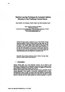
In our quest for a generic classification methodology we first examined plots of packet size against packet interarrival time (IAT) for the two unidirectional flows that make up a single ‘connection’. (We define a unidirectional flow in the conventional sense of a series of packets sharing the same five-tuple (source IP address and port, destination IP address port, and protocol number). We do not timeout flows, except where they exceed the length of the trace (6 hours). From this point in this paper, we will refer to these pairs of unidirectional flows as a bidirectional flow, or just a flow. The IAT/packet size plots exhibit a number of characteristic shapes that we believe are indicative of the application type. Examples of these plots (produced 3 from the Auckland-VI[10]) trace are shown in figure 1. Only four example plots are shown here, however there are other types that that we have not shown due to space limitations. To illustrate the point that the same protocol may carry different traffic types, two different HTTP sessions are included (1(a) and (b)). In the following paragraphs we explain the most likely causes for the major characteristics of these plots. Our analysis is not exhaustive and is primarily intended to illustrate the point that some (but not all) of these characteristics are indicative of the type of application that generated the traffic. For simplicity, we have stated our analysis in the imperative. There were approximately 20,000 flows in the trace we analysed but less than a dozen of these characteristics plot types (plus a some plots that did not fit any characteristic type). Fig 1(a) shows a flow containing a single HTTP request for a large object. There is a single large packet from the server to the client (the HTML GET 3

A colour version of this paper is available at http://www.wand.net.nz/pubs.php.

Client to Server Server to Client

1200

1200

1000

1000

800

600

800

600

400

400

200

200

0 1e-05

0.0001

0.001

0.01

0.1

1

10


1400

Packet size in bytes


1400

0 1e-05

100

0.0001

Time since last packet in flow in seconds

1000

1000 Packet size in bytes


1200

800

600

200

200

0.01

0.1

1

(c) FTP (control)

100

10


600

400


10

800

400

0.001

1

1400

1200

0.0001

0.1

(b) Multiple HTTP 1.1 Requests


0 1e-05

0.01


(a) A single large HTTP Request 1400

0.001

100

0 1e-05

0.0001

0.001

0.01

0.1

1

10


(d) SMTP Mail exchange

Fig. 1. HTTP Packet Interarrival/Size plots

request) and many small packets (the TCP acknowledgements). There are many large packets of the same size (full data packets) from the server to the client. There are also a few smaller packets (partly full data packets) and a single minimum sized packet (an ACK without data) from the server to the client. Fig 1(b) shows a flow containing multiple HTTP requests in a single connection (HTTP 1.1). In addition to the packets of the Fig 1(a) there are additional request packets (mostly ranging between 300 and 600 bytes). Notice the cluster of packets centred roughly around (size = 500, IAT = 0.3s). This type of cluster is typical of protocols in query/reply/query transaction mode and is the result of fetching small objects via HTTP. Finally, note the vertical grouping at approximately IAT = 1.1ms. This is probably the result of the TCP Nagle Algorithm operating to delay the transmission of partly full packets until the previous packet is acked. Fig 1(c) is a similar plot for an FTP control connection. It shows a cluster of points around IAT = 100ms and then a spread of points above that. The cluster is again a query/response/query cluster (but with smaller queries and

100

responses than the multiple HTTP request example). The spread, which ranges up to about a minute, is related to human interaction times required to generate a new command. Because FTP uses a separate connection for data transfer there is no bulk data phase for this flow. The final plot in the set, Fig 1(d), shows a mail transfer using SMTP. Again there is a transaction cluster (but with a wider IAT range, indicating that some queries took longer to resolve than others). There is also a bulk transfer component with large packets. The reason for some of the large packets being 1500 bytes and others being 1004 bytes was investigated at some length. The 1004 byte packets are final packet in a repeated series of transfers. That is, this SMTP session contained 25 transfers of messages requiring five 1500 byte and one 1004 byte packets to transfer. Given SMTP’s multiple recipient feature and the normal variation in length of email addresses in the message header, this is almost certainly spam.

3

Clustering and Classification

While it would be possible to form groups of flows by writing code that was aware of the characteristics we discovered in the IAT/Packet size plots, this approach imposes a high degree of human interpretation in the results. It is also unlikely to be sufficiently flexible to allow the methodology to be used in diverse network types. Machine learning techniques can also be used to cluster the flows present in the data and then to create a classification from the clusters. This is a multiple step process. The data is first divided into flows as described above. A range of attributes are extracted from each flow. These attributes are: – packet size statistics (minimum, maximum, quartiles, minimum as fraction of max and the first five modes) – interarrival statistics – byte counts – connection duration – the number of transitions between transaction mode and bulk transfer mode, where bulk transfer mode is defined as the time when there are more than three successive packets in the same direction without any packets carrying data in the other direction – the time spent: idle (where idle time is the accumulation of all periods of 2 seconds or greater when no packet was seen in either direction), in bulk transfer and in transaction mode These characteristics are then used by the EM clustering algorithm (described in section 3.1 below) to group the flows into a small number of clusters. This process is not a precise one. To refine the clusters we generate classification rules that characterise the clusters based on the raw data. From these rules attributes that do not have a large impact on the classification are identified and removed from the input to the clusterer and the process is repeated. Although it is not discussed further in this paper, the process is also repeated within each cluster, creating sub-clusters of each of the major flow types.

0.25

0.2

0.15

0.1

A

B

0.05

0

0

10

20

30

40

50

60

70

Fig. 2. A two cluster mixture model.

3.1

The EM algorithm for probabilistic clustering

The goal of clustering is to divide flows (instances in the generic terminology of machine learning) into natural groups. The instances contained in a cluster are considered to be similar to one another according to some metric based on the underlying domain from which the instances are drawn. The results of clustering and the algorithms that generate clusters, can typically be described as either “hard” or “soft”. Hard clusters (such as those generated by the simple k-means method [5]) have the property that a given data point belongs to exactly one of several mutually exclusive groups. Soft clustering algorithms, on the other hand, assign a given data point to more than one group. Furthermore, a probabilistic clustering method (such as the EM algorithm [6]) assigns a data point to each group with a certain probability. Such statistical approaches make sense in practical situations where no amount of training data is sufficient to make a completely firm decision about cluster memberships. Methods such as EM [6] have a statistical basis in probability density estimation. The goal is to find the most likely set of clusters given the training data and prior expectations. The underlying model is called a finite mixture. A mixture is a set of probability distributions—one for each cluster—that model the attribute values for members of that cluster. Figure 2 shows a simple finite mixture example with two clusters—each modelled by a normal or Gaussian distribution—based on a single numeric attribute. Suppose we took samples from the distribution of cluster A with probability p and the distribution of cluster B with probability 1 − p. If we made a note of which cluster generated each sample it would be easy to compute the maximum likelihood estimates for the parameters of each normal distribution (the sample mean and variance of the points sampled from A and B respectively) and the mixing probability p. Of course, the whole problem is that we do not know which cluster a particular data point came from, nor the parameters of the cluster distributions. The EM (Expectation-Maximisation) algorithm can be used to find the maximum likelihood estimate for the parameters of the probability distributions in

the mixture model4 . The basic idea is simple and involves considering unobserved latent variables zij . The zij ’s take on values 1 or 0 to indicate whether data point i comes from cluster j’s model or not. The EM algorithm starts with an initial guess for the parameters of the models for each cluster and then iteratively applies a two step process in order to converge to the maximum likelihood fit. In the expectation step, a soft assignment of each training point to each cluster is performed—i.e. the current estimates of the parameters are used to assign cluster membership values according to the relative density of the training points under each model. In the maximisation step, these density values are treated as weights and used in the computation of new weighted estimates for the parameters of each model. These two steps are repeated until the increase in log-likelihood (the sum of the log of the density for each training point) of the data given the current fitted model becomes negligible. The EM algorithm is guaranteed to converge to a local maximum which may or may not be the same as the global maximum. It is normal practice to run EM multiple times with different initial settings for the parameter values, and then choose the final clustering with the largest log-likelihood score. In practical situations there is likely to be more than just a single attribute to be modelled. One simple extension of the univariate situation described above is to treat attributes as independent within clusters. In this case the log-densities for each attribute are summed to form the joint log-density for each data point. This is the approach taken by our implementation5 of EM. In the case of a nominal attribute with v values, a discrete distribution—computed from frequency counts for the v values—is used in place of a normal distribution. Zero frequency problems for nominal attributes can be handled by using the Laplace estimator. Of course it is unlikely that the attribute independence assumption holds in real world data sets. In these cases, where there are known correlations between attributes, various multivariate distributions can be used instead of the simple univariate normal and discrete distributions. Using multivariate distributions increases the number of parameters that have to be estimated, which in turn increases the risk of overfitting the training data. Another issue to be considered involves choosing the number of clusters to model. If the number of clusters in the data is not known a-priori then hold-out data can be used to evaluate the fit obtained by modelling 1, 2, 3, ..., k clusters [4]. The training data can not be used for this purpose because of overfitting problems (i.e. greater numbers of clusters will fit the training data more closely and will result in better log-likelihood scores). Our implementation of EM has an option to allow the number of clusters to be found automatically via cross-validation. Cross-validation is a method for estimating the generalisation performance (i.e. the performance on data that has not been seen during training) of an algorithm based on resampling. The resulting estimates of perfor4

5

Actually EM is a very general purpose tool that is applicable to many maximum likelihood estimation settings (not just clustering). Included as part of the freely available Weka machine learning workbench (http://www.cs.waikato.ac.nz/ml/weka)

mance (in this case the log-likelihood) are often used to select among competing models (in this case the number of clusters) for a particular problem.

4

Cluster Visualisation

The result of clustering is a grouping of flows. By examining the IAT/packet size plots it is possible, given enough thought, to make sense of the clusters produced but this is a difficult process. To aid the interpretation of the meaning of the clusters, we developed a visualisation based on the Kiviat graph[1]. The six toplevel clusters for one of our sample data sets are shown in figure 3. Each graph describes the set of flows in a cluster. The (blue) lines radiating out from the centre point are axes representing each of the attributes we used for clustering. The thick part of the axes represents one standard deviation above and below the mean, the medium thickness lines represent two standard deviations, and the thin lines represent three standard deviations. Note that, in some cases, the axis extends beyond the graph plane and has been truncated. The mean point for each attribute is connected to form the (red) shape in the centre of the graph. Different shapes are characteristic of different traffic profiles. The standard deviation as a percentage of the mean is shown on each axis. This figure gives an indication of how important this attribute is in forming this cluster. If the percentage is high, then this attribute is likely to be a strong classifier. The cluster shown in figure 3(a) contains 59% of the flows in this sample. In this cluster the mean packet size from the server is about 300 bytes and has a large standard deviation. The total number of packets is small (especially remembering the 7 packet overhead of a normal TCP connection). Clients send about 900 bytes of data and servers send an average of about 2300. The duration is short (¡1s) and the flow normally stays in transaction mode. This cluster is mostly typical web traffic, fetching small and medium sized objects, for example HTML pages, icons and other small images. There are two other similar clusters, clusters 3 and 4, shown in Fig 3(d) and (e) respectively. These clusters represent a further 20% of flows. Cluster 4 represents larger objects (with a mean server bytes of about 18000 bytes. In addition to HTTP, quite a lot of SMTP traffic is included in this cluster. The flows in cluster 3 have a significant idle time. These are mostly HTTP 1.1 flows with one or more objects fetched over the same connection. The connection is held open, in the ideal state, for a time after an object is transfered to give the client time to request another object. Cluster five (Fig. 3(f)) contains classic bulk transfer flows. They are short to medium term (a mean of 1m 13s) and transfer a lot of data from the server to the client. Clusters one and two (Fig. 3(b) and (c))are long duration flows with a lot of idle time. Flows in cluster two have many small packets transfered in both directions. These are transaction based with multiple transactions in the flow, separated by significant delays. IMAP and NTP are examples. Cluster one has only a few packets. This is predominantly TCP DNS traffic. We suspect this cluster includes applications where the connection is not correctly terminated.

Proportion of flows in cluster 0: 59% (502857)

Proportion of flows in cluster 1: 4% (41107) 0.768800 (103.08%) duration

0.000001 (10000.00%) idleTime

2338.164400 (140.73%) totalBytes_srv

0.065600 (380.03%) timeInBulk

6.057200 (45.03%) totalPackets_srv

7264.681800 (139.56%) idleTime

7266.705500 (139.51%) duration

1233.052500 (89.82%) totalBytes_srv

0.000001 (10000.00%) timeInBulk


0.219000 (188.86%) stateChanges

921.019400 (55.06%) totalBytes_client

0.019000 (718.42%) stateChanges


140.675700 (42.49%) PSMeanClient

6.613600 (33.68%) totalPackets_client

103.114000 (50.25%) PSMeanClient


308.066100 (94.17%) PSMeanServer

0.129600 (127.31%) MeanIATServer

0.226400 (95.98%) IATvarClient

0.213400 (107.22%) IATvarServer

0.125500 (111.71%) MeanIATClient

186.342100 (60.16%) PSMeanServer

1650.884700 (147.52%) IATvarClient

1766.130400 (153.38%) MeanIATServer

(a)

(b)


7252.984500 (142.58%) idleTime


2408.096600 (168.08%) timeInBulk

52016.719300 (229.46%) totalBytes_srv


8.140600 (305.41%) stateChanges


124.188300 (93.84%) PSMeanClient


625.666800 (65.15%) PSMeanServer

608.487100 (190.48%) IATvarClient

280.016700 (295.87%) MeanIATServer

603.323900 (198.61%) IATvarServer

253.750500 (228.71%) MeanIATClient

41.813200 (85.96%) idleTime

44.239300 (81.74%) duration


0.704400 (157.13%) stateChanges


145.455400 (56.51%) PSMeanClient


349.135600 (98.40%) PSMeanServer




8.944800 (99.17%) IATvarServer

(d)



1.609700 (142.23%) timeInBulk

18131.339300 (116.83%) totalBytes_srv


0.866600 (73.09%) stateChanges


144.548600 (87.51%) PSMeanClient


645.696000 (72.45%) PSMeanServer


4534.395700 (148.00%) totalBytes_srv

10.385800 (256.54%) timeInBulk

(c)

1.697100 (150.48%) idleTime

1744.444200 (153.06%) MeanIATClient

1635.730900 (149.14%) IATvarServer


0.664800 (81.26%) IATvarServer


58.330800 (124.11%) idleTime

73.396300 (118.66%) duration

50.863900 (139.71%) timeInBulk


3.835500 (119.24%) stateChanges


269.225100 (117.59%) PSMeanClient


760.954700 (60.66%) PSMeanServer

5.113800 (111.49%) IATvarClient

126298.499900 (383.46%) totalBytes_srv


3.823500 (127.79%) IATvarServer

(e)

(f) Fig. 3. Clusters 1 (a), 2 (b) and 4 (c)


Fig. 4. Ports Across Clusters

5

Validation

We are still actively developing the methodology. As part of this process we have undertaken four types of validation. We looked at the stability of the clusters within different segments of a single trace, comparing the clusters produced from the whole trace with those produced from half of the trace. Secondly, we compared two traces from different, but similar, locations (the University of Auckland and The University of Waikato). While there were differences in the statistics of the attributes, both these exercises yielded the same basic set of clusters, as shown by their Kiviat graphs. Next we examined the distribution of ports across the clusters. Because port numbers are indicative of the application in use we expected ports to be focused on particular clusters. The graphic in Fig 4 shows this distribution for the 20 most common ports. Each stack of bars represents a port with the most common ports on the left and the least common on the right. The width of the bar represents the number of flows with that port type, on a logarithmic scale. Each band represents a cluster, with the largest cluster (cluster 0) at the top, and the smallest (cluster 2) at the bottom. The distribution of ports across clusters is less differentiated than we expected. There are several reasons for this. First it should be noted that, the log scale of figure 4 (which is necessary to allow the visualisation to show more than just the two or three dominant port types) creates a false impression of the distribution of ports. The second, and more important reason is one we alluded to in the introduction, we just under estimated its significance. HTTP is the predominant traffic type in these traces. HTTP has a wide range of uses and consequently there is a significant amount of HTTP traffic in all clusters. Finally, we examined whether the algorithm was assigning flows of particular port types to clusters differently than a random assignment would. This analysis, which we can not present here for space reasons, indicated that for most ports

there was good discrimination between clusters but for a few, there was not. IMAP is one example where the discrimination was poor. It seems that, the clustering is generally doing a good job of grouping flows together by their traffic type (bulk transfer, small transactions, multiple transactions etc.) but that individual applications behave more differently across different connections than we had expected. Even given these reasons, the clustering does not currently meet our needs and we are continuing to develop the approach, especially through the derivation of new attributes that we believe will further discriminate between applications. The existence of idle time at the end of a connection is one example.

6

Conclusion

The initial results of the methodology appear promising. The clusters are sensible and the clustering and classification algorithms indicate that a good fit has been obtained to the data. Initial analysis indicates that the clusters are stable over a range of different data with the same overall characteristics. The existing clusters provide an alternative way to disaggregate a packet header stream and we expect it to prove useful in traffic analysis that focuses on a particular traffic type. For example, simulation of TCP optimisations for high performance bulk transfer. However, further work is required to fully meet our initial goal of clustering traffic into groups that a network manager would recognise as related to the particular application types on their network.

References 1. Kolence, K., Kiviat, P.: Software Unit Profiles and Kiviat Figures. ACM SIGMETRICS, Performance Evaluation Review, Vol. 2, No. 3 September (1973) 2–12 2. Witten, I,. and Frank, E., Data Mining: Practical Machine Learning Tools and Techniques with Java Implementations. Morgan Kaufmann (2000) 3. Hastie, T., Tibshirani, R., and Friedman, J., The Elements of Statistical Learning: Data Mining, Inference, and Prediction Springer-Verlag (2001) 4. Smyth, P., Clustering Using Monte Carlo Cross-Validation Proceedings of the Second International Conference on Knowledge Discovery and Data Mining AAAI Press (1996) 126–133 5. Hartigan, J., Clustering Algorithms John Wiley (1975) 6. Dempster, A., Laird, N., and Rubin, D., Maximum Likelihood from Incomplete Data Via the EM Algorithm Journal of the Royal Statistical Society Series B, Vol. 30, No. 1 (1977) 1–38 7. http://www.nlanr.net/ 8. http://www.wand.net.nz/ 9. Claffy, K., Braun, H.-W. and Polyzos, G. Internet traffic flow profiling Applied Network Research, San Diego Supercomputer Center (1994) Available at: http://www.caida.org/outreach/papers/ 10. Mochalski, K., Micheel, J. and Donnelly, S. Packet Delay and Loss at the Auckland Internet Access Path Proceedings of the PAM2002 Passive and Active Measurement Conference, Fort Collins, Colorado USA, (2002)