Using Machine Learning Techniques to Combine ... - CiteSeerX

Using Machine Learning Techniques to Combine Forecasting Methods Ricardo Prudêncio and Teresa Ludermir Centro de Inform´ atica, Universidade Federal de Pernambuco Caixa Postal 7851 - CEP 50732-970 - Recife (PE) - Brazil {rbcp, tbl}@cin.ufpe.br Abstract. We present here an original work that uses machine learning techniques to combine time series forecasts. In this proposal, a machine learning technique uses features of the series at hand to define adequate weights for the individual forecasting methods being combined. The combined forecasts are the weighted average of the forecasts provided by the individual methods. In order to evaluate this solution, we implemented a prototype that uses a MLP network to combine two widespread methods. The experiments performed revealed significantly accurate forecasts.

1

Introduction

Time series forecasting has been widely used to support decision-making. Combining forecasts from different forecasting methods is a procedure commonly used to improve forecasting accuracy [1]. An approach that uses knowledge for combining forecasts is based on expert systems, such as the Rule-Based Forecasting system [2]. This system defines a weight for each individual method according to the features of the series being forecasted. The combined forecasts are then the weighted average of the forecasts provided by the individual methods. Despite its good results, developing rules in this context may be unfeasible, since good experts are not always available [3]. In order to minimize the above difficulty, we proposed the use of machine learning techniques for combining forecasts. In the proposed solution, each training example stores the description of a series (i.e. the series features) and the combining weights that empirically obtained the best forecasting performance for the series. A machine learning technique uses a set of such examples to relate time series features and adequate combining weights. In order to evaluate the proposed solution, we implemented a prototype that uses MLP neural networks [4] to define the weights for two widespread methods: the Random Walk and the Autoregressive model [5]. The prototype was evaluated in a large set of series and compared to benchmarking forecasting procedures. The experiments revealed that the forecasts generated by the prototype were significantly more accurate than the benchmarking forecasts. Section 2 presents some methods for combining forecasts, followed by section 3 that describes the proposed solution. Section 4 brings the experiments and results. Finally section presents some conclusions and the future work. G.I. Webb and Xinghuo Yu (Eds.): AI 2004, LNAI 3339, pp. 1122–1127, 2004. c Springer-Verlag Berlin Heidelberg 2004

Using Machine Learning Techniques to Combine Forecasting Methods

2

1123

Combining Forecasts

The combination of forecasts is a well-established procedure for improving forecasting accuracy [1]. Procedures that combine forecasts often outperform the individual methods that are used in the combination [1]. The linear combination of K methods can be described as follows. Let Zt (t = 1, . . . , T ) be the available data of a series Z and let Zt (t = T + 1, . . . , T + H) be the H future values to be forecasted. Each method k uses the available data to k,t . The combined forecasts Z C,t are defined as: generate its forecasts Z C,t = Z

K

k,t wk ∗ Z

(1)

k=1

The combining weights wk (k = 1, . . . , K) are numerical values that indicate the contribution of each individual method in the combined forecasts. Eventually constraints are imposed on the weights in such a way that: K

wk = 1 and wk ≥ 0

(2)

k=1

Different approaches for defining combining weights can be identified [1]. An very simple approach is to define equal weights (i.e. wk = 1/K), which is usually referred as the Simple Average (SA) combination method. Despite its simplicity, the SA method has shown to be robust in the forecasting of different series. A more sophisticated approach for defining the combining weights was proposed by [6], by treating the linear combination of forecasts within the regression framework. In this context, the individual forecasts are viewed as the explanatory variables and the actual values of the series as the response variable. An alternative approach for the combination of forecasts is based on the development of expert systems, such as the Rule-Based Forecasting system [2]. The rules deployed by the system use the time series features (such as length, basic trend,...) to modify the weight associated to each model. In the experiments performed using the system, the improvement in accuracy over the SA method has shown to be significant.

3

The Proposed Solution

As seen, expert systems have been successfully used to combine forecasts. Unfortunately, the knowledge acquisition in these systems depends on the availability of human forecasting experts. However, good forecasting experts are often scarce and expensive [3]. In order to minimize this difficulty, the use of machine learning techniques is proposed here to define the weights for combining forecasts. The proposed solution is closely related to previous works that used learning algorithms to select forecasting methods [3][7][8]. In our work, the learning algorithms are used to define the best linear combination of methods.

1124

R. Prudêncio and T. Ludermir

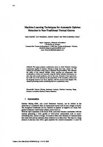
Input Problem (I): Time Series Data + Contextual Information

-

Time Series Features (y) FE

-

IC

6

- Combining Weights: w1 (I), . . . , wK (I)

Training Examples (E) DB Fig. 1. System’s architecture

Figure 1 presents the architecture of a system following our solution. The system has two phases: training and use. In the training phase, the Intelligent Combiner (IC) uses a supervised algorithm to acquire knowledge from a set of examples E in the Database (DB). Each example ei ∈ E stores the values of P features Y1 , . . . , YP for a particular series and the adequate combining weights w1 , ..., wK for K methods. Each feature Yj (j = 1, . . . , P ) is either: (1) a descriptive statistic or; (2) a contextual information. The IC module uses the set E to build a learner L that associates the features and the combining weights. In the use phase, the system’s user provides an input problem I (i.e. time series data and contextual information). The Feature Extractor (FE) module extracts the description y = Y1 (I), . . . , YP (I) (i.e. the time series features) for the input problem. The learner L uses these values to predict the adequate weights for the input problem: L(y) = {w1 (I), . . . , wK (I)}. In order to verify the viability of the proposal, we implemented a prototype which define the combining weights for K = 2 methods: the Random Walk (RW) and the Auto-Regressive model (AR) [5]. The prototype was applied to forecast the yearly series of the M3-Competition [9], which provides a large set of time series related to certain economic and demographic domains and represent a convenient sample for expository purposes. 3.1

The Feature Extractor

In this module, the following features were used to describe the yearly series of the M3-Competition: 1. Length of the time series (L): number of observations of the series; 2. Basic Trend (BT): slope of the linear regression model; 3. Percentage of Turning Points (TP): Zt is a turning point if Zt−1 < Zt > Zt+1 or Zt−1 > Zt < Zt+1 . This feature measures the oscillation in a series; 4. First Coefficient of Autocorrelation (AC): large values of this feature suggest that the value of the series at a point influences the value at the next point; 5. Type of the time series (TYPE): it is represented by 5 categories, micro, macro, industry, finances and demographic. The first four features are directly computed using the series data and TYPE in turn is a contextual information provided by the authors of M3-Competition.


3.2

1125

The Intelligent Combiner

The IC module uses the Multi-Layer Perceptron (MLP) network [4] (one hidden layer) as the learner. The MLP input layer has 9 units that represent the time series features. The first four input units receive the values of the numeric features (i.e. L, BT, TP, AC). The feature TYPE was represented by 5 binary attributes (either 1 or 0 value), each one associated to a different category. The output layer has two nodes that represent the weights associated to the RW and AR models. In order to ensure that the final combining weights are non-negative and sum to one (see eq. 2), the outputs of the MLP are normalized. The MLP training is performed by the standard BackPropagation (PB) algorithm [4] and follows the benchmark training rules provided in Proben [10]. The BP algorithm was implemented using the Neural Network Toolbox [11]. 3.3

The Database

An important aspect to be considered in the prototype is the generation of the training examples. In order to construct an example using a specific series Z, the following tasks have to be performed. First, the series data is divided into two parts: the fit period Zt (t = 1, . . . , T ) and the test period Zt (t = T +1, . . . , T +H). The test period in our prototype consists on the last H = 6 years of the series and the fit period consists on the remaining data. The fit data is used to calibrate the RW and AR models. The calibrated models are used to generate the individual k,t (k = 1, 2)(t = T + 1, ..., T + 6) for the test data. forecasts Z In the second task, we defined the combining weights wk (k = 1, 2) that C,t (t = minimize the Mean Absolute Error (MAE) of the combined forecasts Z T + 1, ..., T + 6). This task can be formulated as an optimization problem: Minimize: T +6 T +6 2 1 1 k,t | M AE(ZC,t ) = |Zt − ZC,t | = |Zt − wk ∗ Z 6 6 t=T +1

Subject to:

2

t=T +1

wk = 1 and wk ≥ 0

(3)

k=1

(4)

k=1

This optimization problem was treated using a line search algorithm implemented in the Optimization toolbox for Matlab [12]. In the third task, the features (see section 3.1) are extracted for the fit period of the series. The features of the fit period and the weights that minimized the forecasting error in the test period are stored in the DB as a new example.

4

Experiments and Results

In this section, we initially describe the experiments performed to select the best number of hidden nodes for the MLP. In these experiments, we used the 645

1126

R. Prudêncio and T. Ludermir Table 1. Training results Number of Hidden Nodes 2 4 6 8 10

SSE Training Average Deviation 65.15 1.87 64.16 1.97 64.22 1.81 64.13 2.28 2.62 64.37

SSE Validation Average Deviation 69.46 0.80 69.49 0.87 69.34 0.86 0.67 69.29 69.56 1.03

SSE Test Average Deviation 68.34 1.03 67.78 1.20 1.28 67.14 66.74 1.35 67.54 1.32

yearly series of the M3-Competition [9] and hence 645 training examples. The set of examples was equally divided into training, validation and test sets. We trained the MLP using 2, 4, 6, 8 and 10 nodes (30 runs for each value). The optimum number of nodes was chosen as the value that obtained the lowest average SSE error on the validation set. Table 1 summarizes the MLP training results. As it can be seen, the optimum number of nodes according to the validation error was 8 nodes. The gain obtained by this value was also observed in the test set. We further investigated the quality of the forecasts that were generated using the weights suggested by the selected MLP. In order to evaluate the forecasting performance across all series i ∈ test set, we considered the Percentage Better (PB) measure [13]. Given a method Q, the PB measure is computed as follows: P BQ = 100 ∗

T +6 1 δQit m i∈test

(5)

t=T +1

where δQit =

1, if |eRit | < |eQit | 0, otherwise

(6)

In the above definition, R is a reference method that serves for comparison. The eQit is the forecasting error obtained by Q in the i-th series at time t, and m is the number of times in which |eRit | < |eQit |. Hence, P BQ indicates in percentage terms, the number of times that the error obtained by the method R was lower than the error obtained using the method Q. Values lower than 50 indicate that the method Q is more accurate than the reference method. The P B measure was computed for three reference methods. The first one is merely to use RW for forecasting all series and the second is to use AR for all series. The third reference method is the Simple Average (SA) combination. The table summarizes the PB results over the 30 runs of the best MLP. As it can be seen, the average PB measure was lower than 50% for all reference methods, and the confidence intervals suggest that the obtained gain is statistically significant.

5

Conclusion

In this work, we proposed the use of machine learning techniques to define the best linear combination of forecasting methods. We can point out contributions


1127

Table 2. Comparative forecasting performance measured by PB Reference Method RW AR SA

PB Measure Average Deviation Conf. Interv. (95%) 42.20 0.26 [42.11; 42.29] [40.04; 40.36] 40.20 0.44 43.24 1.45 [42.72; 43.76]

of this work to two fields: (1) in time series forecasting, since we provided a new method for that can be used to combine forecasts; (2) in machine learning, since we used its concepts and techniques in a problem which was not tackled yet. In order to evaluate the proposal, we used MLP networks to combine two forecasting models. The experiments performed revealed encouraging results. Some modifications in the current implementation may be performed, such as augmenting the set of time series features and optimizing the MLP design.

References 1. De Menezes, L. M., Bunn, D. W. and Taylor, J. W.: . Review of guidelines for the use of combined forecasts. European Journal of Operational Research, 120 (2000) 190-204. 2. Collopy, F. and Armstrong, J. S.: Rule-based forecasting: development and validation of an expert systems approach to combining time series extrapolations. Management Science, 38(10) (1992) 1394-1414. 3. Arinze, B.: Selecting appropriate forecasting models using rule induction. OmegaInternational Journal of Management Science, 22(6) (1994) 647-658. 4. Rumelhart, D.E., Hinton, G.E. and Williams, R.J.: Learning representations by backpropagation errors. Nature, 323 (1986) 533-536. 5. Harvey, A.: Time Series Models. MIT Press, Cambridge, MA (1993) 6. Granger, C.W.J. and Ramanathan, R.: Improved methods of combining forecasts. Journal of Forecasting, 3 (1984) 197204. 7. Venkatachalan, A.R. and Sohl, J.E.: An intelligent model selection and forecasting system. Journal of Forecasting, 18 (1999) 167-180. 8. Prudêncio, R.B.C. and Ludermir, T.B.: Meta-Learning Approaches for Selecting Time Series Models. Neurocomputing Journal, 61(C) (2004) 121-137. 9. Makridakis, S. and Hibon, M.: The M3-competition: results, conclusions and implications. International Journal of Forecasting, 16(4) (2000) 451-476. 10. Prechelt, L.: Proben 1: a set of neural network benchmark problems and benchmarking rules, Tech. Rep. 21/94, Fakultat fur Informatik, Karlsruhe (1994). 11. Demuth, H. and Beale, M.:. Neural Network Toolbox for Use with Matlab, The Mathworks Inc, (2003). 12. The Mathworks, Optimization Toolbox User’s Guide, The Mathworks Inc. (2003). 13. Flores, B.E.: Use of the sign test to supplement the percentage better statistic. International Journal of Forecasting, 2 (1986) 477-489.