Manifold Reconstruction in Arbitrary Dimensions using Witness ... - Inria

Manifold Reconstruction in Arbitrary Dimensions using Witness Complexes Jean-Daniel Boissonnat

Leonidas J. Guibas

Steve Y. Oudot

INRIA, Geometrica 2004, route des lucioles 06902 Sophia-Antipolis

Computer Science Dept. Stanford University Stanford, CA 94305

Computer Science Dept. Stanford University Stanford, CA 94305

[email protected]

[email protected]

ABSTRACT It is a well-established fact that the witness complex is closely related to the restricted Delaunay triangulation in low dimensions. Specifically, it has been proved that the witness complex coincides with the restricted Delaunay triangulation on curves, and is still a subset of it on surfaces, under mild sampling assumptions. Unfortunately, these results do not extend to higher-dimensional manifolds, even under stronger sampling conditions. In this paper, we show how the sets of witnesses and landmarks can be enriched, so that the nice relations that exist between both complexes still hold on higher-dimensional manifolds. We also use our structural results to devise an algorithm that reconstructs manifolds of any arbitrary dimension or co-dimension at different scales. The algorithm combines a farthest-point refinement scheme with a vertex pumping strategy. It is very simple conceptually, and does not require the input point sample W to be sparse. Its time complexity is bounded by c(d)|W |2 , where c(d) is a constant depending solely on the dimension d of the ambient space. Categories and Subject Descriptors: I.3.5 [Computer Graphics]: Curve, surface, solid, and object representations General Terms: Algorithms, Theory. Keywords: Witness complex, restricted Delaunay triangulation, manifold reconstruction, sampling conditions.

1. INTRODUCTION A number of areas of Science and Engineering deal with point clouds lying on submanifolds of Euclidean spaces. Such data can be either collected through measurements of natural phenomena, or generated by simulations. Given a finite set of sample points W , presumably drawn from an unknown manifold S, the goal is to retrieve some information about S from W . This manifold learning problem, which is at the core of non-linear dimensionality reduction techniques [25 27], finds applications in many areas, including

Permission to make digital or hard copies of all or part of this work for personal or classroom use is granted without fee provided that copies are not made or distributed for profit or commercial advantage and that copies bear this notice and the full citation on the first page. To copy otherwise, to republish, to post on servers or to redistribute to lists, requires prior specific permission and/or a fee. SCG’07, June 6–8, 2007, Gyeongju, South Korea. Copyright 2007 ACM 978-1-59593-705-6/07/0006 ...$5.00.

[email protected]

machine learning [4], pattern recognition [26], scientific visualization [28], image or signal processing [22], and neural computation [16]. The nature of the sought-for information is very application-dependent, and sometimes it is enough to inquire about the topological invariants of the manifold, a case in which techniques such as topological persistence [8 13 29] offer a nice mathematical framework. However, in many situations it is desirable to construct a simplicial complex with the same topological type as the manifold, and close to it geometrically. This problem has received a lot of attention from the computational geometry community, which proposed elegant solutions in low dimensions, based on the use of the Delaunay triangulation D(W ) of the input point set W – see [6] for a survey. In these methods, the output complex is extracted from D(W ), and it is equal or close to D S (W ), the Delaunay triangulation of W restricted to the manifold S. What makes the Delaunay-based approach attractive is that, not only does it behave well on practical examples, but its performance is guaranteed by a sound theoretical framework. Indeed, the restricted Delaunay triangulation is known to provide good topological and geometric approximations of smooth or Lipschitz curves in the plane and surfaces in 3space, under mild sampling conditions [1 2 5]. Generalizing these ideas to arbitrary dimensions and codimensions is difficult however, because a given point set W may sample well various manifolds with different homotopy types, as illustrated in Figure 1. To overcome this issue, it has been suggested to strengthen the sampling conditions, so that they can be satisfied by only one class of manifolds sharing the same topological invariants [12 17 20]. In some sense, this is like choosing arbitrarily between the possible reconstructions, and ignoring the rest of the information carried by the input. Moreover, the new sets of conditions on the input are so strict that they are hardly satisfiable in practice, thereby making the contributions rather theoretical. Yet [12 17 20] contain a wealth of relevant ideas and results, some of which are used in this paper. A different and very promising approach [7 9 21 23], reminiscent of topological persistence, builds a one-parameter family of complexes that approximate S at various scales. The claim is that, for sufficiently dense W , the family contains a long sequence of complexes carrying the same homotopy type as S. In fact, there can be several such sequences, each one corresponding to a plausible reconstruction – see Figure 1. Therefore, performing a reconstruction on W boils down to finding the long stable sequences in the

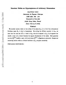
Figure 1: A helical curve drawn on a torus (top). Any dense sampling of the curve is also a dense sampling of the torus. To deal with this ambiguity, the algorithm of [21] builds a sequence of complexes (bottom) approximating the input at various scales, and maintains their Betti numbers (top).

one-parameter family of complexes. This approach to reconstruction stands in sharp contrast with previous work in the area. In [7 9 23], the family of complexes is derived from the α-offsets of the input W , where α ranges from zero to infinity. The theoretical guarantees of [7] hold in a very wide setting, since W is assumed to be a sufficiently dense sampling of a general compact set. In [21], the family is given by the witness complex of L relative to W , or C W (L) for short, where L is a subset of W constructed iteratively, starting with L = ∅, and inserting each time the point of W lying furthest away from L. It is known that C W (L) coincides with D S (L) on smooth curves, and is still included in it on smooth surfaces [3 21]. The assumptions on L in [21] are more stringent than the ones on W , but this is not an issue since L is generated by the algorithm. Unfortunately, the structural results of [3 21] do not hold in higher dimensions, which makes it very unlikely that the algorithm works on any manifold S of dimension greater than two. The reason is that the normals of D S (L) can be arbitrarily wrong if DS (L) contains badly-shaped simplices, called slivers [12]. As a consequence, C W (L) may not be included in D S (L), which may not be homotopy equivalent to S [24]. This is true even if W and L satisfy strong sampling conditions, such as being arbitrarily dense uniform samples of S. In this paper, we show how to enrich W and L in order to make the structural results of [3 21] hold for higherdimensional manifolds. To each point p ∈ L we assign a non-negative weight ω(p), so that D S (L) and C W (L) are now replaced by their weighted versions, DωS (L) and CωW (L). The idea of assigning weights to the vertices comes from [10], where it was used to remove slivers from 3-dimensional Delaunay triangulations. This sliver removal technique was extended to higher dimensions by Cheng et al. [12], who

showed that, under sufficient sampling conditions on L, there exists a distribution of weights ω such that DωS (L) is homeomorphic to S. Our main result is that, for the same distribution of weights and under similar conditions on L, CωW (L) is included in DωS (L), for all W ⊆ S. Combined with the fact that CωS (L) contains DωS (L), we get that CωS (L) = DωS (L), which is homeomorphic to S. This is a generalization of the result of [3] to higher-dimensional manifolds. It is not quite practical since W has to be equal to S. In the more realistic case where W is a finite subset of S, we enlarge it by replacing its points by balls of radius ζ. For sufficiently large ζ, this ζ enlarged set W ζ contains S, and hence DωS (L) ⊆ CωW (L). ζ And if ζ is not too large, then CωW (L) is still included in ζ DωS (L). Thus, we obtain CωW (L) = DωS (L) under sufficient conditions on W, L, ζ. Here again, the condition on L is stringent, but the one on W is mild. These structural results suggest combining the method of [21] with the sliver exudation technique of [10], in order to make it work on higher-dimensional manifolds. Our combination is the simplest possible: at each iteration of the algorithm, we insert a new point p in L, compute its best ζ possible weight, and update CωW (L). This algorithm is very simple conceptually, and to some extent it can be viewed as a dynamic version of the algorithm of [12], where the Delaunay triangulation of W would be constructed progressively as the weights of the points of W are computed. This raises a number of questions, such as whether the weight assignment process removes all the slivers from the vicinity of DωS (L), since some of the weights are assigned in early stages of the course of the algorithm. We prove that all slivers are inζ deed removed at some point, and that consequently CωW (L) is homeomorphic to S, provided that W is a dense enough sampling of S. Our assumption on W is much less stringent than the one used in [12], which makes our algorithm more practical. On the other hand, our assumption that S is a smooth manifold is stronger than the one of [7], but we get stronger ζ guarantees, namely CωW (L) is homeomorphic to S, whereas the complex of [7] is only homotopy equivalent to S. Observe also that the witness complex is always embedded in the ambient space Rd , which is not the case of the nerve of an offset. This is important if one wants to do further processing on the reconstruction. By considering the α-shape of W instead of the nerve of its α-offset, the authors of [7] get rid of this issue. Nevertheless, they cannot get rid of the so-called curse of dimensionality because, as α varies from zero to infinity, the α-complex spans the entire d-dimensional “ ” Delaunay triangulation of W , whose size d is Θ |W |d /2e . In contrast, the witness complex can be maintained by considering only the κ(d) nearest neighbors in L of each point of W , which reduces the time complex` ´ ity of our algorithm to O c(d)|W |2 , where κ(d) and c(d) are constants depending solely on d. This is worse than the bound of [12] (c(d)|W | log |W |) since we cannot benefit from the sparseness assumption on W , which is essential for the correctness of the algorithm of [12]. The outline of the paper is as follows: after recalling the necessary background in Section 2, we present our main structural result (Theorem 3.1) in Section 3, and we introduce our reconstruction algorithm in Section 4.

2. BACKGROUND AND DEFINITIONS 2.1 Manifolds and samples The ambient space isqRd , d ≥ 3, equipped with the usual Pd 2 Euclidean norm kpk = i=1 pi . All manifolds considered

in this paper are compact closed submanifolds of Rd , of dimension two or more. The case of curves has already been addressed1 in [21]. The reach of a manifold S, or rch(S) for short, is the minimum distance of a point on S to the medial axis of S. All manifolds in this paper are assumed to have a positive reach. This is equivalent to saying that they are C 1 -continuous, and that their normal vector field satisfies a Lipschitz condition. Given a (finite or infinite) subset L of a manifold S, and a positive parameter ε, L is an ε-sample of S if every point of S is at Euclidean distance at most ε to L, and L is ε-sparse if the pairwise Euclidean distances between the points of L are at least ε. Note that an ε-sparse sample of a compact set is always finite. Parameter ε is sometimes made adaptative in the literature [1], its value depending on the distance to the medial axis of the manifold.

2.2 Simplex shape Given k + 1 points p0 , · · · , pk ∈ Rd , [p0 , · · · , pk ] denotes the k-simplex of vertices p0 , · · · , pk . The geometric realization of this simplex is the convex hull of p0 , · · · , pk , which has dimension k if the vertices are affinely independent. Following [11], we call sliver measure of [p0 , · · · , pk ] the ratio2 : %([p0 , · · · , pk ]) =

vol([p0 , · · · , pk ]) , min{kpi − pj k, 0 ≤ i < j ≤ k}k

(1)

where vol([p0 , · · · , pk ]) denotes the volume of the convex hull of p0 , · · · , pk in Rk . In the special case where k = 1, we have %([p0 , p1 ]) = 1 for any edge [p0 , p1 ]. We extend the notion of sliver measure to the case k = 0 by imposing %([p0 ]) = 1 for any vertex p0 . Given %¯ ≥ 0, simplex [p0 , · · · , pk ] is said to be k a %¯-sliver if %([p0 , · · · , pk ]) < %¯ /k!. For sufficiently small %¯, this means that the volume of the simplex is small compared to the volume of the diametral k-ball of its shortest edge. As a result, the simplex is badly-shaped. Note however that having a large sliver measure does not always mean being well-shaped. Take an isoceles triangle t of base b and height √ h·b h h ≥ b 2 3 . Its sliver measure is %(t) = 2b 2 = 2b . Reducing b while keeping h constant makes t arbitrarily skinny but %(t) arbitrarily large – t is called a dagger in the literature [10]. Parameter %¯ is called the sliver bound in the sequel.

2.3 Weighted points, Delaunay triangulation, and witness complex Given a finite point set L ⊂ Rd , a distribution of weights on L is a non-negative real-valued function ω : L → [0, ∞). ω(u) The quantity maxu∈L,v∈L\{u} ku−vk is called the relative

amplitude of ω. Given p ∈ Rd , the weighted distance from p to some weighted point v ∈ L is kp − vk2 − ω(v)2 . This is actually not a metric, since it is not symmetric. Whenever 1

The results of [21] apply to Lipschitz curves in the plane, but they can be extended to smooth curves in higher dimensions in a straightforward manner. 2 This definition generalizes the one of [10] to higher dimensions. It departs from the definition of [12], which introduced a bug in the proof of Lemma 10 of the same paper.

the relative amplitude of ω is less than 12 , the points of L have non-empty cells in the weighted Voronoi diagram of L, and in fact each point of L belongs to its own cell [10]. Given a finite point set L ⊂ Rd , and a distribution of weights ω on L, we denote by Dω (L) the weighted Delaunay triangulation of L [19]. For any simplex σ of Dω (L), Vω (σ) denotes the face of the weighted Voronoi diagram of L that is dual to σ. Moreover, given any subset X of Rd , we call DωX (L) the weighted Delaunay triangulation of L restricted to X. In the special case where all the weights are equal, Dω (L) coincides with the standard Euclidean Delaunay triangulation, and is therefore noted D(L). Similarly, Vω (σ) becomes V(σ), and DωX (L) becomes D X (L). Definition 2.1. Let W, L ⊆ Rd be such that L is finite, and let ω be a distribution of weights on L. • Given a point w ∈ W and a simplex σ = [p0 , · · · , pk ] with vertices in L, w ω-witnesses σ if p0 , · · · , pk are among the k + 1 nearest neighbors of w in the weighted metric, that is, ∀i ∈ {0, · · · , k}, ∀q ∈ L \ {p0 , · · · , pk }, kw − pi k2 − ω(pi )2 ≤ kw − qk2 − ω(q)2 . • The ω-witness complex of L relative to W , or CωW (L) for short, is the maximum abstract simplicial complex with vertices in L, whose faces are ω-witnessed by points of W . This definition comes from [14 15]. From now on, W will be referred to as the set of witnesses, and L as the set of landmarks. In the special case where all the weights are equal, CωW (L) coincides with the witness complex for the standard Euclidean norm, and is therefore noted C W (L). Given a distribution of weights ω on L, for any simplex σ = [p0 , · · · , pk ] of DωW (L) and any point w ∈ W lying on the weighted Voronoi face dual to σ, we have that w is a ωwitness of σ and that kw−pi k2 −ω(pi )2 = kw−pj k2 −ω(pj )2 ∀i, j ∈ {0, · · · , k}. Hence, w is also a ω-witness of all the subsimplices of σ, which therefore belong to CωW (L). Corollary 2.2. For any W, L ⊆ Rd with L finite, for any ω : L → [0, ∞), DωW (L) ⊆ CωW (L). DωW (L) is sometimes called the strong witness complex of L relative to W in the literature [15]. Given a distribution of weights ω on L, we say that the weighted points of L lie in general position if no point of Rd is equidistant to d + 2 points of L in the weighted metric, and if no d + 1 points on the convex hull of L are coplanar. Under this assumption, every simplex of Dω (L) has dimension at most d. Theorem 2.3 (Thm. 2 and §3 of [14]). Let W, L ⊆ Rd be such that L is finite. Let also ω be any distribution of weights on L, such that the weighted point set L lies in general position. Let σ be a simplex with vertices in L. If σ and all its subsimplices are ω-witnessed by points of W , then σ belongs to Dω (L). In other words, CωW (L) is a subcomplex of Dω (L). Moreover, the dual weighted Voronoi face of σ intersects the convex hull of the ω-witnesses of σ and its subsimplices. It is always possible to perturb the points of L or their weights infinitesimally, so as to make them lie in general position. Therefore, in the rest of the paper we assume implicitely that the weighted point set L is in general position. On 1- and 2-dimensional manifolds, the unweighted witness complex is closely related to the unweighted restricted Delaunay triangulation [3 21], which provides good topological and geometric approximations [1 2]. However, as proved

in [24], these properties do not extend to higher-dimensional manifolds, even under stronger sampling conditions: Theorem 2.4 (see [24]). For any positive constant µ < 1/3, there exists a closed and compact hypersurface S of positive reach in R4 , and an Ω(ε)-sparse O(ε)-sample L of S, with ε = µ rch(S), such that D S (L) is not homotopy equivalent to S. The constants hidden in the Ω and O notations are absolute and do not depend on µ. In addition, for any δ > 0, there exists a δ-sample W of S such that C W (L) neither contains nor is contained in D S (L). Furthermore, W can be made indifferently finite or infinite. The proof of this theorem builds on an example of [12, §11]. The intuition is that, when D S (L) contains slivers, it is possible to make its normals turn by a large angle (say π/2) by perturbing the points of L infinitesimally. Then, the combinatorial structure of D S (L) can change arbitrarily under small perturbations of S. The consequence is that D S (L) may not be homotopy equivalent to S, and it may not contain all the simplices of C W (L) either. In addition, as emphasized in [21], for any k ≥ 2, the k-simplices of D S (L) may have arbitrarily small cells in the restricted Voronoi diagram of L of order k + 1, which implies that they may not be witnessed in W if ever W ( S.

2.4 Weighted cocone complex At any point p on a manifold S, there exist a tangent space T (p) and a normal space N (p). These two subspaces of Rd are orthogonal, and their direct sum is Rd . For any angle value θ ∈ [0, π/2], we call θ-cocone of S at p, or Kθ (p) for short, the cone of semi-aperture θ around the tangent space of S at p: Kθ (p) = {q ∈ Rd | ∠(pq, T (p)) ≤ θ}. The name cocone refers to the fact that Kθ (p) is the complement of a cone of semi-aperture π2 − θ around the normal space of S at p. Given an angle θ ∈ [0, π/2], a manifold S, a finite point set L ⊂ S, and a distribution of weights ω : L → [0, ∞), the weighted θ-cocone complex of L, noted Kθω (L), is the subcomplex of Dω (L) made of the simplices whose dual weighted Voronoi faces intersect the θ-cocone of at least one of their vertices. This means that a simplex [p0 , · · · , pk ] of Dω (L) belongs to Kθω (L) if, and only if, its dual weighted Voronoi face intersects Kθ (p0 ) ∪ · · · ∪ Kθ (pk ). Note that the cones in [12] are defined around approximations of the tangent spaces of S at the points of L. However, the results of [12] hold a fortiori when the approximations of the tangent spaces are error-free, which is the case here. Theorem 2.5 (Lemmas 13, 14, 18 of [12]). For any sliver bound %¯ > 0, there exists a constant c%¯ > 0 such that, for any manifold S, for any ε-sparse 2ε-sample L of S with ε ≤ c%¯ rch(S), and for any ω : L → [0, ∞) of relative ampliπ/32 π/32 tude less than 12 , if Kω (L) has no %¯-sliver, then Kω (L) coincides with DωS (L), which is homeomorphic to S. It is also proved in [12] that, for any ω ¯ ∈ (0, 1/2), there exists a distribution of weights ω on L, of relative amplitude at π/32 most ω ¯ , that removes all %¯-slivers from Kω (L). This is true provided that %¯ is sufficiently small compared to ω ¯, and that ε ≤ c%¯ rch(S) (as in Theorem 2.5, the choice of %¯ influences the bound on ε). The results of [12] hold in fact in the slightly more general setting where ε is a (non-uniform) 1-Lipschitz function, everywhere bounded by a fraction of the distance to the medial axis of S – see [12, §13].

2.5

Useful results

The following results, adapted from [12 20], will be used in the sequel: Lemma 2.6 (Lemma 6 of [20]). Let S be a manifold, and let p, q ∈ S be such that kp − qk < rch(S). Then, the 2 Euclidean distance from q to T (p) is at most 2kp−qk . rch(S) Lemma 2.7 (Lemma 2 of [12]). Let S be a manifold and θ ∈ [0, π/2] an angle value. Let v ∈ S and p ∈ Kθ (v) be such that kp − vk < rch(S). Then, the” Euclidean distance “ from p to S is at most sin θ +

kp−vk 2 rch(S)

kp − vk.

Lemma 2.8 (Lemma 3 of [12]). Let S be a manifold and θ ∈ [0, π/2) an angle value. Let L be an ε-sample of S, with ε < 49 (1 − sin θ)2 rch(S). For any ω : L → [0, ∞) of relative amplitude less than 12 , for any v ∈ L and any 3ε . p ∈ Kθ (v) ∩ Vω (v), we have kp − vk ≤ 1−sin θ

3.

STRUCTURAL RESULTS

In this section, ω ¯ ∈ (0, 1/2) and %¯ > 0 are fixed constants. For any k ≥ 0, we define c1 (k) = 4 (1 + 2¯ ω + k(1 + 3¯ ω )) and c2 (k) = 4 (3 + 6¯ ω + 2k(1 + 3¯ ω )). Let S be a manifold in Rd , W a (finite or infinite) δ-sample of S in Rd , and L a (finite) εsparse ε-sample of W , for two parameters δ, ε to be specified later on. Note that L is an (ε + δ)-sample of S. According to Theorem 2.4, C W (L) may not coincide with D S (L), even under strong assumptions on δ, ε. Specifically: • some simplices of D S (L) may not belong to C W (L) if W does not span S entirely. Our solution to this problem is to enlarge the set of witnesses, in order to make it cover S. More precisely, we dilate W by a ball of radius ζ centeredSat the origin, so that the set of witnesses is now W ζ = w∈W B(w, ζ). For ζ ≥ δ, this set contains S, ζ

ζ

hence DωS (L) ⊆ DωW (L) ⊆ CωW (L). • some simplices of C W (L) may not belong to D S (L) if the latter contains %¯-slivers. To remedy this problem, we assign non-negative weights to the landmarks, so that DS (L) and C W (L) are now replaced by their weighted versions, DωS (L) and CωW (L). Given any angle value θ ∈ (0, π/2), our main structural result (Theorem 3.1) states that, under sufficient conditions on δ, ε, ζ, Kθω (L) conζ tains CωW (L) for any ω : L → [0, ∞) of relative ampliζ tude at most ω ¯ . Therefore, CωW (L) ⊆ DωS (L) whenever π/32 π θ ≤ 32 and ω removes all %¯-slivers from Kω (L), by Theorem 2.5.

Theorem 3.1. Given any angle value θ ∈ (0, π/2), if δ, ε, ζ satisfy the following conditions: 5(1−ω ¯ 2 ) sin θ H1 2(1−ω¯52 ) sin θ δ ≤ ε ≤ 2 rch(S), 2(1−ω ¯ 2 ) sin θ+5c2 (d)) ( i h 2(1−ω ¯ 2 ) sin θ ε , H2 ζ ∈ δ, 5 ζ

ζ

then DωS (L) ⊆ DωW (L) ⊆ CωW (L) ⊆ Kθω (L) for any distribution of weights ω on L of relative amplitude at most ω ¯ . If in addition θ ≤ π/32, ε ≤ c%¯ rch(S), and ω is such π/32 that Kω (L) contains no %¯-sliver3 , then Theorem 2.5 imζ ζ π/32 plies that DωW (L) = CωW (L) = Kω (L) = DωS (L), which is homeomorphic to S. 3 As mentioned after Theorem 2.5, such distributions of weights exist, provided that %¯ is sufficiently small.

H1 requires that W is dense compared to L, which must be dense compared to rch(S). This is very similar in spirit to the condition of [21]. H2 bounds the dilation parameter ζ. The smaller the angle θ of semi-aperture of the cocones, the smaller ε must be for Kθω (L) to contain DωS (L), and the ζ smaller ζ must be for Kθω (L) to contain CωW (L). Condition S Wζ ζ ≥ δ ensures that Dω (L) ⊆ Cω (L). In the special case where W = S (which implies δ = 0) and ζ = 0, H2 and the left-hand side of H1 become void, and the theorem states that CωS (L) coincides with DωS (L) for a suitable distribution of weights ω : L → [0, ∞), provided that L is an ε-sparse ε-sample of S, for a small enough ε. This is an extension of the result of Attali et al. [3] to higher dimensions, with an additional sparseness condition on L. This condition is mandatory for the existence of a suitable ω on manifolds of dimension three or higher [10 12]. The general case of Theorem 3.1 allows to have W ( S, which is more practical. Another useful property, stated as Theorem 3.2 below, is that the weighted witness complex actually includes the weighted cocone complex, for any distribution of weights of relative amplitude at most ω ¯ , provided that ζ is sufficiently large compared to ε. Note that this condition on ζ is incompatible4 with H2: as a consequence, two different values of ζ have to be used in order to bound Kθω (L), as emphasized in our algorithm – see Section 4. π , and if δ, ε satisfy Condition Theorem 3.2. If θ ≤ 32 7 sin θ H1 of Theorem 3.1, then, for any ζ ≥ 2(1−sin ε, for any θ)

ω : L → [0, ∞) of relative amplitude at most ω ¯ , Kθω (L) ⊆ ζ ζ DωW (L) ⊆ CωW (L). The rest of Section 3 is devoted to the proofs of Theorems 3.1 and 3.2, and we give an overview below.

Overview of the proofs The proof of Theorem 3.1 is given in Section 3.1. Showing ζ ζ that DωS (L) ⊆ DωW (L) ⊆ CωW (L) is in fact easy: since W ζ is a δ-sample of S, W contains S whenever ζ ≥ δ, which is guaranteed by H2; it follows immediately that DωS (L) ⊆ ζ ζ DωW (L), which by Corollary 2.2 is included in CωW (L) for ζ any ω : L → [0, ∞). Showing that CωW (L) ⊆ Kθω (L) requires more work, but the core argument is very simple, namely: the Euclidean distances between a point of S and its k nearest landmarks in the weighted metric are bounded (Lemma 3.4). From this fact we derive some bounds on ζ the Euclidean distances between the simplices of CωW (L) and their ω-witnesses (Lemma 3.5). These bounds are then used to show that the ω-witnesses of a simplex σ lie in the θ-cocones of the vertices of σ, from which we deduce that ζ CωW (L) ⊆ Kθω (L) (Lemma 3.6). The proof of Theorem 3.2 is given in Section 3.2. Intuitively, if L is a sufficiently dense sampling of S, then, for any simplex σ ∈ Kθω (L) and any vertex v of σ such that Vω (σ) ∩ Kθ (v) 6= ∅, the points of Vω (σ) ∩ Kθ (v) lie close to T (v) and hence close to S. Therefore, they belong to W ζ whenever ζ is large enough, which implies that ζ ζ σ ∈ DωW (L) ⊆ CωW (L). 4 Indeed, the upper bound on ζ in H2 is always smaller than the lower bound on ζ in Theorem 3.2.

3.1

Proof of Theorem 3.1

As explained above, all we have to do is to show that, ζ whenever Conditions H1–H2 are satisfied, CωW (L) is inθ cluded in Kω (L) for any ω : L → [0, ∞) of relative amplitude at most ω ¯ . We will use the following bound on the weights: Lemma 3.3. Under Condition H1 of Theorem 3.1, for any v ∈ L and any ω : L → [0, ∞) of relative amplitude at most ω ¯ , ω(v) is at most 2¯ ω (ε + δ). Proof. Let v ∈ L, and let Sv be the connected component of S containing v. Consider the cell V(v) of v in the unweighted Voronoi diagram of L. Since L is an (ε + δ)sample of S, Sv ∩V(v) is contained in the ball B(v) of center v and radius ε + δ. By H1, the radius of this ball is at most rch(S), hence we have Sv ∩B(v) ( Sv . This implies that the boundary of V(v) intersects Sv . Let p be a point of intersection. There is a point u ∈ L such that kp − uk = kp − vk, which is at most ε + δ. Hence, kv − uk ≤ 2(ε + δ). We deduce that ω(v) ≤ ω ¯ kv − uk ≤ 2¯ ω (ε + δ), since ω ¯ bounds the relative amplitude of ω. Here is now the core argument of the proof of Theorem 3.1: Lemma 3.4. Under Condition H1 of Theorem 3.1, for any ω : L → [0, ∞) of relative amplitude at most ω ¯ , for any p ∈ S, and for any k ≤ d, the Euclidean distance between p and its (k + 1)th nearest landmark in the weighted metric is at most rk = (1 + 2¯ ω + 2k(1 + 3¯ ω )) (ε + δ). Proof. The proof is by induction on k. Assume first that k = 0. Let v1 ∈ L be the nearest neighbor of p in the weighted metric, and u ∈ L the nearest neighbor of p in the Euclidean metric. Observe that u may or may not be equal to v1 . Since L is an (ε+δ)-sample of S, kp−uk is at most ε+ δ. Moreover, we have kp − v1 k2 − ω(v1 )2 ≤ kp − uk2 − ω(u)2 , which gives kp−v1 k2 ≤ kp−uk2 +ω(v1 )2 −ω(u)2 ≤ (ε+δ)2 + ω(v1 )2 − ω(u)2 . Note that −ω(u)2 is non-positive, and that ω(v1 )2 is at most 4¯ ω 2 (ε + δ)2 , by Lemma 3.3. Therefore, 2 kp − v1 k ≤ (1 + 4¯ ω 2 )(ε + δ)2 ≤ (1 + 2¯ ω )2 (ε + δ)2 , which proves the lemma in the case k = 0. Assume now that k ≥ 1, and that the result holds up to k − 1. Let v1 , · · · , vk denote the k nearest landmarks of p in the weighted metric. By induction, we have {v1 , · · · , vk } ⊂ B (p, rk−1 ). Moreover, by the case k = 0 above, for any i ≤ k we have S ∩ Vω (vi ) ⊆ B(vi , (1 + 2¯ ω )(ε + δ)), which is included in B(p, rk−1 + (1 + 2¯ ω )(ε + δ)). Let Sp be the connected component of S that contains p. It follows from H1 that rk−1 + (1 + 2¯ ω )(ε + δ) ≤ rch(S), hence we have S ∩ B(p, rk−1 + (1 + 2¯ ω )(ε + δ)) ( Sp , which implies two things: first, v1 , · · · , vk belong to Sp ; second, their weighted Voronoi cells do not cover Sp entirely. As a consequence, S Sp must intersect the boundary of ki=1 (S ∩ Vω (vi )). Let q be a point of intersection: q lies on the bisector hyperplane between some vi and some point v ∈ L \ {v1 , · · · , vk }, i.e. q ∈ Vω (vi ) ∩ Vω (v). By the case k = 0 above, kq − vi k and kq − vk are at most (1 + 2¯ ω )(ε + δ). Moreover, we have kp − vi k ≤ rk−1 , by induction. Therefore, kp − vk ≤ kp − vi k + kvi − qk + kq − vk ≤ rk−1 + 2(1 + 2¯ ω )(ε + δ). Since v ∈ L\{v1 , · · · , vk }, we have kp−vk+1 k2 −ω(vk+1 )2 ≤ kp−vk2 −ω(v)2 , where vk+1 is the (k+1)th nearest landmark of p in the weighted metric. Hence, kp − vk+1 k2 ≤ kp − vk2 + ω(vk+1 )2 ≤ (kp − vk + ω(vk+1 ))2 , which is at most (rk−1 +2(1+2¯ ω )(ε+δ)+2¯ ω (ε+δ))2 = rk2 , by Lemma 3.3.

Using Lemma 3.4, we can bound the Euclidean distances ζ between the simplices of CωW (L) and their ω-witnesses. Our bounds depend on quantities c1 (k), c2 (k), defined at the top of Section 3: Lemma 3.5. Under Conditions H1–H2 of Theorem 3.1, for any ω : L → [0, ∞) of relative amplitude at most ω ¯ , for ζ any k-simplex σ of CωW (L) (k ≤ d), and for any vertex v of σ, we have: (i) for any ω-witness c ∈ W ζ of σ, kc − vk ≤ c1 (k) ε, (ii) for any subsimplex σ 0 ⊆ σ and any ω-witness c0 ∈ W ζ of σ 0 , kc0 − vk ≤ c2 (k) ε. ζ

Proof. Let σ be a k-simplex of CωW (L). By definition, there is a point c ∈ W ζ that ω-witnesses σ. This means that the vertices of σ are the (k +1) nearest landmarks of c in the weighted metric. Unfortunately, we cannot apply Lemma 3.4 directly to bound the Euclidean distance between c and its (k+1) nearest landmarks in the weighted metric, because c may not belong to S. However, since c ∈ W ζ , there is some point w ∈ W ⊆ S such that c ∈ B(w, ζ). By Lemma 3.4, the ball B(w, rk ) contains at least (k + 1) landmarks. Thus, at least one landmark u in B(w, rk ) does not belong to the k nearest landmarks of c in the weighted metric. This means that, for any l ≤ k + 1, kc − vl k2 − ω(vl )2 ≤ kc − uk2 − ω(u)2 , where vl denotes the lth nearest landmark of c in the weighted metric. It follows that kc − vl k2 ≤ kc − uk2 + ω(vl )2 − ω(u)2 ≤ (kc − uk + ω(vl ))2 , which by Lemma 3.3 is at most (kc − uk + 2¯ ω (ε + δ))2 . Since kc − uk ≤ kc−wk+kw−uk ≤ ζ +rk , we get kc−vl k ≤ ζ +rk +2¯ ω (ε+δ), which by H1–H2 is bounded by c1 (k) ε. Since this is true for any l ≤ k + 1, the Euclidean distance between c and any vertex of σ is at most c1 (k) ε. This proves (i). ζ Let σ 0 be any subsimplex of σ. Since σ belongs to CωW (L), 0 0 ζ 0 σ is ω-witnessed by some point c ∈ W . Let w ∈ W ⊆ S be such that c0 ∈ B(w0 , ζ). According to Lemma 3.4, the Euclidean distance between w 0 and its nearest landmark u0 in the weighted metric is at most r0 = (1+2¯ ω )(ε+δ). Hence, kc0 − u0 k ≤ ζ + r0 . Let v10 be the nearest landmark of c0 in the weighted metric. We have kc0 − v10 k2 ≤ kc0 − u0 k2 + ω(v10 )2 − ω(u0 )2 ≤ (kc0 − u0 k + ω(v10 ))2 , which is at most (ζ + r0 + 2¯ ω (ε + δ))2 , by Lemma 3.3. Since c0 ω-witnesses σ 0 , 0 v1 is a vertex of σ 0 and hence also a vertex of σ. Thus, for any vertex v of σ, we have kc0 − vk ≤ kc0 − v10 k + kv10 − vk, which by (i) is at most ζ + r0 + 2¯ ω (ε + δ) + 2c1 (k) ε. This quantity is bounded by c2 (k) ε, since under H1–H2 δ and ζ are at most ε. This proves (ii). ζ

We can now show that CωW (L) ⊆ Kθω (L), which concludes the proof of Theorem 3.1: Lemma 3.6. Under Conditions H1–H2 of Theorem 3.1, for any distribution of weights ω : L → [0, ∞) of relative ζ amplitude at most ω ¯ , for any k-simplex σ of CωW (L) (k ≤ θ d), and for any vertex v of σ, Vω (σ) ∩ K (v) 6= ∅. As a ζ consequence, CωW (L) ⊆ Kθω (L). ζ

Proof. Let σ be a k-simplex of CωW (L), and let v ∈ L be any vertex of σ. If k = 0, then σ = [v]. Since the relative amplitude of ω is at most ω ¯ < 12 , v belongs to its weighted Voronoi cell Vω (v). And since v belongs to Kθ (v), we have Vω (v) ∩ Kθ (v) 6= ∅, which proves the lemma in the case k = 0.

Assume now that 1 ≤ k ≤ d. By Lemma 3.5 (ii), for any simplex σ 0 ⊆ σ, for any ω-witness c0 of σ 0 , we have kc0 − vk ≤ c2 (k) ε ≤ c2 (d) ε. Since c0 ∈ W ζ , there is a point w0 ∈ W ⊆ S such that kw 0 − c0 k ≤ ζ, which implies that kw 0 − vk ≤ ε (c2 (d) + ζ/ε). This quantity is at most rch(S), by H1–H2, hence the Euclidean distance from w 0 ε2 (c2 (d) + ζ/ε)2 , by Lemma 2.6. It to T (v) is at most 2 rch(S) follows that the Euclidean distance from c0 to T (v) is at most ε2 (c2 (d) + ζ/ε)2 . This holds for any ω-witness c0 ∈ ζ + 2 rch(S) ζ

W ζ of any simplex σ 0 ⊆ σ. Since σ is a simplex of CωW (L), Theorem 2.3 tells us that σ belongs to Dω (L), and that the dual weighted Voronoi face of σ intersects the convex hull of the ω-witnesses of the subsimplices of σ. Let p be a point of intersection. Since the ω-witnesses of the subsimplices of σ ε2 (c2 (d) + ζ/ε)2 from T (v), do not lie farther than ζ + 2 rch(S) neither does p, which belongs to their convex hull. Let us now give a lower bound on kp−vk, which will allow us to conclude afterwards. Since the dimension k of σ is at least one, σ has at least two vertices. Hence, there exists at least one point u ∈ L \ {v} such that kp − vk2 − ω(v)2 = kp − uk2 −ω(u)2 , which gives kp−vk2 = kp−uk2 +ω(v)2 −ω(u)2 . Since ω ¯ bounds the relative amplitude of ω, we have ω(u)2 ≤ 2 ω ¯ ku − vk2 . Moreover, ω(v)2 is non-negative. Hence, kp − vk2 ≥ kp − uk2 − ω ¯ 2 ku − vk2 . By the triangle inequality, 2 we obtain kp − vk ≥ (kp − vk − ku − vk)2 − ω ¯ 2 ku − vk2 , which gives kp − vk ≥ 12 (1 − ω ¯ 2 )ku − vk. This implies that kp − vk ≥ 12 (1 − ω ¯ 2 )ε, since L is ε-sparse. ε2 To conclude, p is at most ζ + 2 rch(S) (c2 (d) + ζ/ε)2 away 2 1 from T (v), and at least 2 (1 − ω ¯ )ε away from v, in the + Euclidean metric. Therefore, sin ∠(vp, T (v)) ≤ (1−2ζ ω ¯ 2 )ε ε (1−ω ¯ 2 )rch(S)

(c2 (d) + ζ/ε)2 , which is at most sin θ, by H1–

H2. As a consequence, p belongs to Kθ (v). Now, recall that p is a point of Vω (σ). Hence, Vω (σ) ∩ Kθ (v) 6= ∅, which means that σ is a simplex of Kθω (L). Since this is true for ζ any k-simplex σ of CωW (L) (k ≤ d), and since, by Theorem ζ 2.3, CωW (L) is included in Dω (L), which has no simplex of dimension greater than d because the weighted point set L ζ lies in general position, CωW (L) is included in Kθω (L).

3.2

Proof of Theorem 3.2

Let σ be a simplex of Kθω (L). By definition, the dual weighted Voronoi face of σ intersects the θ-cocone of at least one vertex v of σ. Let c be a point of intersection. Since L is an (ε + δ)-sample of S, with ε + δ < 94 (1 − 3(ε+δ) sin θ)2 rch(S), Lemma 2.8 states that kc − vk ≤ 1−sin , θ which is less than rch(S) since by assumption we have ε + θ rch(S).“ Therefore, by Lemma δ < 1−sin 3 ” 2.7, we have

3(ε+δ) 3(ε+δ) kq 0 − ck ≤ 1−sin sin θ + 2(1−sin , where q 0 is a θ θ) rch(S) point of S closest to c. Since W is a δ-sample of S, there exists some point w ∈“W such that kq 0 − wk” ≤ δ. Hence,

kc − wk ≤ δ +

3(ε+δ) 1−sin θ

sin θ +

3(ε+δ) 2(1−sin θ) rch(S)

, which is at

ζ

most ζ by hypothesis. It follows that c ∈ W , and hence ζ that σ belongs to DωW (L). This concludes the proof of Theorem 3.2.

4. MANIFOLD RECONSTRUCTION In this section, we use our structural results in the context of manifold reconstruction. From now on, we fix ω ¯ = 14 and π θ = 32 , and we set %¯ to an arbitrarily small positive value. We give an overview of the approach in Section 4.1, then we present the algorithm in Section 4.2, and we prove its correctness in Section 4.3. Our theoretical guarantees are discussed in Section 4.4. In Section 4.5, we give some details on how the various components of the algorithm can be implemented. These details are then used in Section 4.6 to bound the space and time complexities of the algorithm.

4.1 Overview of the approach

ζ2

simplices of the star of p in CωW (L). After the pumping, ζ1 ζ2 ω(p) is increased to ωp , and CωW (L), CωW (L) are updated. The algorithm terminates when L = W . The output is the ζ1 one-parameter family of complexes CωW (L) built throughout the process. It is in fact sufficient to output the diagram of their Betti numbers, computed on the fly using the persistence algorithm of [29]. With this diagram, the user can determine the scale at which to process the data: it is then easy to generate the corresponding subset of weighted landmarks (the points of W have been sorted according to their order of insertion in L, and their weights have been stored) and to rebuild its weighted witness complex relative to W ζ1 .

Let W be a finite input point set drawn from some unknown manifold S, such that W is a δ-sample of S, for some unknown δ > 0. Imagine we were able to construct an εsparse ε-sample L of W , for some ε ≤ c%¯ rch(S) satisfying Condition H1 of Theorem 3.1. Then, Theorems 3.1 and ζ1 π/32 3.2 would guarantee that DωS (L) ⊆ CωW (L) ⊆ Kω (L) ⊆ ζ2 CωW (L) for any distribution of weights of relative ampli2 π tude at most ω ¯ , where ζ1 = 2(1−ω¯5 ) sin θ ε = 38 sin 32 ε and 7 sin π/32 ζ2 = 2(1−sin π/32) ε. We could then apply the pumping strat-

Input: W ⊂ Rd finite. Init: Let L := ∅; ε := +∞; ζ1 := +∞; ζ2 := +∞; While L ( W do Let p := argmaxw∈W minv∈L kw − vk; // p is chosen arbitrarily in W if L = ∅ L := L ∪ {p}; ω(p) := 0; ε := maxw∈W minv∈L kw − vk; 7 sin π/32 π ζ1 := 83 sin 32 ε; ζ2 := 2(1−sin π/32) ε; ζ1

ζ2

egy of [10] to CωW (L), which would remove all %¯-slivers ζ2 π/32 from CωW (L) (and hence from Kω (L)) provided that %¯ is ζ1 sufficiently small. As a result, CωW (L) would coincide with S Dω (L) and be homeomorphic to S, by Theorem 2.5. Unfortunately, since δ and rch(S) are unknown, finding an ε ≤ c%¯ rch(S) that provably satisfies H1 can be difficult, if not impossible. This is why we combine the above approach with the multi-scale reconstruction scheme of [21], which generates a monotonic sequence of samples L ⊆ W . Since L keeps growing during the process, ε keeps decreasing, eventually satisfying H1 if δ is small enough. At that stage, ζ1 CωW (L) becomes homeomorphic to S, and thus a plateau ζ1 appears in the diagram of the Betti numbers of CωW (L), showing the homology type of S – some examples can be found in [21]. Note that the only assumption made on the input point set W is that it is a δ-sample of some manifold, for some small enough δ. In particular, W is not assumed to be a sparse δ-sample. As a result, W may well-sample several manifolds S1 , · · · , Sl , as it is the case for instance in the example of Figure 1. In such a situation, the values δ1 , · · · , δl for which W is a δi -sample of Si differ, and they generate distinct ζ1 plateaus in the diagram of the Betti numbers of CωW (L) – see Figure 1.

4.2 The algorithm The input is a finite point set W ⊂ Rd . Initially, L = ∅ and ε = ζ1 = ζ2 = +∞. At each iteration, the point p ∈ W lying furthest away5 from L in the Euclidean metric is inserted in L and pumped. Specifically, once p has been appended to L, its weight ω(p) is set to zero, and ε is set to maxw∈W minv∈L kw − vk. ζ1 ζ2 CωW (L) and CωW (L) are updated accordingly, ζ1 and ζ2 being defined as in Section 4.1. Then, p is pumped: the pumping procedure Pump(p) determines the weight ωp of p that maximizes the minimum sliver measure among the 5

At the first iteration, since L is empty, p is chosen arbitrarily in W .

ζ2

Update CωW (L) and CωW (L); ω(p) := Pump (p); ζ2 ζ1 Update CωW (L) and CωW (L); End while ζ1 Output: the sequence of complexes CωW (L) obtained after every iteration of the While loop. Figure 2: Pseudo-code of the algorithm. The pseudo-code of the algorithm is given in Figure 2. π/32 The pumping procedure is the same as in [12], with Kω (L) W ζ2 replaced by Cω (L). Given a point p just inserted in L, of weight ω(p) = 0, Pump(p) progressively increases the weight of p up to ω ¯ min{kp − v||, v ∈ L \ {p}}, while maintaining ζ2 the star of p in CωW (L). The combinatorial structure of the star changes only at a finite set of event times. Between consecutive event times, the minimum sliver measure among the simplices of the star is constant and therefore computed once. In the end, the procedure returns an arbitrary value ωp in the range of weights that maximized the minimum sliver measure in the star of p.

4.3

Theoretical guarantees

Assume that the input point set W is a δ-sample of some unknown manifold S. For any i > 0, let L(i), ω(i), ε(i), ζ1 (i), ζ2 (i) denote respectively L, ω, ε, ζ1 , ζ2 at the end of the ith iteration of the main loop of the algorithm. Since L(i) grows with i, ε(i) is a decreasing function of i. Moreover, since the algorithm always inserts in L the point of W lying furthest away from L, it is easily seen that L(i) is an ε(i)-sparse ε(i)-sample of W [21, Lemma 4.1]. ζ1 (i)

W S Theorem 4.1. Cω(i) (L(i)) coincides with Dω(i) (L(i)) and is homeomorphic to S whenever ε(i) ≤ c%¯ rch(S) satisfies H1, which eventually happens during the course of the algorithm if δ is small enough.

The proof of the theorem uses the following intermediate result, whose proof (omitted here) is roughly the same as in Section 8 of [12]:

Lemma 4.2. Whenever δ ≤ ε(i) ≤

2rch(S) 7d−1

− δ, the star of

long enough to be detected by the user or some statistical method applied in a post-processing step. If W samples p(i) in contains no %¯-sliver. several manifolds, then several plateaus may appear in the diagram: each one of them shows a plausible reconstruction, Proof of Theorem 4.1. Let i > 0 be an iteration depending on the scale at which the data set W is processed. such that ε(i) ≤ c%¯ rch(S) satisfies H1. Then, ζ1 (i) = Observe that the structural results of Section 3 still hold6 7 sin π/32 2(1−ω ¯ 2 ) sin θ ε(i) satisfies H2, and ζ2 (i) = 2(1−sin π/32) ε(i) 5 if we relax the assumption on W and allow its points to lie satisfies the hypothesis of Theorem 3.2. Since W is a δslightly off the manifold, at a Hausdorff distance of δ. This sample of S by assumption, and since L(i) is an ε(i)-sparse gives a deeper meaning to Theorem 4.1, which now guaranS ε(i)-sample of W , Theorems 3.1 and 3.2 imply that Dω(i) (L(i)) ⊆ tees that the algorithm generates a plateau whenever there π/32 W ζ1 (i) W ζ2 (i) Cω(i) (L(i)) ⊆ Kω(i) (L(i)) ⊆ Cω(i) (L(i)). Let us show exists a manifold S that is well-sampled by L and that passes π/32 close to the points of W . This holds in particular for small that Kω(i) (L(i)) contains no %¯-sliver, which by Theorem 2.5 deformations S of the manifold S0 from which the points ζ2 (i) W will give the result. In fact, we will prove that Cω(i) (L(i)) of W have been drawn: the consequence is that the topoπ/32 logical features of S0 (connected components, handles, etc.) contains no %¯-sliver, which is sufficient because Kω(i) (L(i)) ⊆ are captured progressively by the algorithm, by decreasing W ζ2 (i) Cω(i) (L(i)). Since ε(i) satisfies H1, we have δ ≤ ε(i) ≤ order of size in the ambient space. For instance, if S0 is a 2rch(S) − δ. Therefore, Lemma 4.2 guarantees that the star double torus whose handles have significantly different sizes, 7d−1 W ζ2 (i) then the algorithm first detects the larger handle, generatof p(i) in Cω(i) (L(i)) contains no %¯-sliver. However, this ing a plateau with β0 = β2 = 1 and β1 = 2, then later on W ζ2 (i) does not mean that Cω(i) (L(i)) itself contains no %¯-sliver, it detects also the smaller handle, generating a new plateau because some of the points of L(i) were pumped at early with β0 = β2 = 1 and β1 = 4. This property, illustrated in stages of the course of the algorithm, when the assumption the experimental section of [21], enlarges greatly the range of Lemma 4.2 was not yet satisfied. of applications of our method. Let i0 ≤ i be the first iteration such that ε(i0 ) ≤ 2rch(S) − Note finally that our theoretical guarantees still hold if 7d−1 ζ1 ζ2 ζ1 ζ2 δ. For any iteration j between i0 and i, we have ε(j) ≤ CωW (L) and CωW (L) are replaced by DωW (L) and DωW (L) 2rch(S) ε(i0 ) ≤ 7d−1 − δ and ε(j) ≥ ε(i) ≥ δ, hence Lemma 4.2 respectively. This means that the algorithm can use indifferguarantees that the pumping procedure removes all %¯-slivers ently the weak witness complex or the strong witness comW ζ2 (j) plex, with similar theoretical guarantees. from the star of p(j) in Cω(j) (L(j)) at iteration j. For any W ζ2 (i) Cω(i) (L(i))

ζ2

k between j and i, the update of CωW (L) after the pumping of p(k) may modify the star of p(j). However, since the pumping of p(k) only increases its weight, the new simplices in the star of p(j) belong also to the star of p(k), which contains no %¯-sliver, by Lemma 4.2. Therefore, the star of W ζ2 (i) (L(i)) still contains no %¯-sliver. p(j) in Cω(i) Consider now an iteration j ≤ i0 − 1. Since ε(j) is greater than 2rch(S) − δ, we cannot ensure that the star of p(j) in 7d−1 ζ2 (j)

W Cω(j)

(L(j)) contains no %¯-sliver. However, we claim that ζ2 (i)

W the points of L(i) that are neighbors of p(j) in Cω(i) (L(i)) were inserted in L on or after iteration i0 . Indeed, for any such neighbor q, there is a point c ∈ W ζ2 (i) that ω(i)witnesses edge [p(j), q]. According to Lemma 3.5 (i), kc − p(j)k and kc − qk are at most c1 (1) ε(i). Hence, we have kp(j) − qk ≤ kp(j) − ck + kc − qk ≤ 2c1 (1) ε(i). Now, recall that L(i0 −1) is ε(i0 −1)-sparse, where ε(i0 −1) > 2rch(S) −δ, 7d−1 which by H1 is greater than 2c1 (1) ε(i). It follows that q cannot belong to L(i0 −1), since p(j) does. Hence, the star of W ζ2 (i) q in Cω(i) (L(i)) contains no %¯-sliver. Since this is true for ζ2 (i)

W (L(i)), the star of p(j) does any neighbor q of p(j) in Cω(i) not contain any %¯-sliver either. This concludes the proof of Theorem 4.1.

4.4 Discussion Theorem 4.1 guarantees the existence of a plateau in the ζ1 diagram of the Betti numbers of CωW (L), but it does not tell exactly where this plateau is located in the diagram, because δ and rch(S) are unknown. Nevertheless, it does give a guarantee on the length of the plateau, which, in view of H1, is of the order of (a rch(S) − b δ), where a, b are two constants. Hence, for sufficiently small δ, the plateau is

4.5

Details of the implementation

Before we can analyze the complexity of the algorithm, we need to give some details on how its various components can be implemented.

4.5.1

Update of the witness complex

Although the algorithm is conceptually simple, its imζ plementation requires to be able to update CωW (L), where ζ ∈ {ζ1 , ζ2 }. This task is significantly more difficult than updating CωW (L), mainly because W ζ is not finite, which makes it impossible to perform the ω-witness test of Definition 2.1 on every single point of W ζ individually. However, since we are working in Euclidean space Rd , for any w ∈ W it is actually possible to perform the ω-witness test on the whole ball B(w, ζ) at once. Each time a point is inserted ζ in L or its weight is increased, CωW (L) is updated by iterating over the points w ∈ W and performing the ω-witness test on B(w, ζ). This test boils down to intersecting B(w, ζ) with the weighted Voronoi diagrams of L of orders 1 through d + 1. In the space of spheres Rd+1 , this is equivalent to intersecting a vertical cylinder of base B(w, ζ) with the cells of an arrangement of |L| hyperplanes, which is a costly operation. Fortunately, as shown below, we can restrict ourselves to constructing the arrangement of the hyperplanes of the κ(d) nearest landmarks of w in the Euclidean metric, where κ(d) = (2 + 2c1 (d))d . This means that we do not actually ζ maintain CωW (L), but another complex C, which might not ζ contain CωW (L) nor be contained in it. Nevertheless, 6

ζ

W ζ still covers S when ζ ≥ δ, and the proof that CωW (L) ⊆ Kθω (L) holds the same, with an additional term δ in the bounds of Lemmas 3.3 through 3.6.

ζ(i)

W Lemma 4.3. C(i) coincides with Cω(i) (L(i)) whenever ε(i) satisfies H1.

Proof. Let w be a point of W , and let Λ(w) ⊆ L(i) denote the set of its κ(d) nearest landmarks in the Euclidean metric. For any point c ∈ B(w, ζ(i)) and any positive integer k ≤ d, Lemma 3.5 (i) ensures that the k + 1 nearest landmarks of c in the weighted metric, p0 , · · · , pk , belong to B(c, c1 (d)ε(i)). Since kw − ck ≤ ζ(i), p0 , · · · , pk belong to B(w, r(i)), where r(i) = ε(i) (c1 (d) + ζ(i)/ε(i)). Now, L(i) is ε(i)-sparse, hence the points of L(i) ∩ B(w, r(i)) are centers of pairwise-disjoint balls of radius ε(i)/2. These balls are included in B (w, r(i) + ε(i)/2), thus their number is at most (1 + 2r(i)/ε(i))d = (1 + 2c1 (d) + 2ζ(i)/ε(i))d , which is bounded by κ(d) since ζ(i) ≤ ζ2 (i) < ε(i)/2. Therefore, p0 , · · · , pk belong to Λ(w). As a result, in the weighted metric, the k + 1 nearest neighbors of c in Λ(w) are the same as its k + 1 nearest neighbors in L(i). Since this is true for any w ∈ W and any c ∈ B(w, ζ(i)), and since all the balls of radius ζ(i) centered at the points of W are tested at each update of the W ζ(i) (L(i)). complex, C(i) coincides with Cω(i) It follows from this lemma that our guarantees on the outζ put of the algorithm still hold if CωW (L) is replaced by C. Note also that, since any arrangement of κ(d) hyperplanes ` ´ 2 in Rd+1 has O κ(d)d+1 = dO(d ) cells [18], each point of 2

W generates at most dO(d ) simplices in C. It follows that 2 the size of our complex is bounded by |W |dO(d ) . The same bound clearly holds for the time spent updating C after a point insertion or a weight increase, provided that the κ(d) 2 nearest landmarks of a witness can be computed in dO(d ) time. In practice, we maintain the lists of κ(d) nearest landmarks of the witnesses in parallel to C. Each time a new point is inserted in L, the list of each witness is updated in O(κ(d)) time as we iterate over all the witnesses to update C. Using these lists, we can retrieve the κ(d) nearest 2 landmarks of any witness in time O(κ(d)) = dO(d ) .

4.5.2

Pumping procedure

As mentioned in Section 4.2, only a finite number of events occur while a point p ∈ L is being pumped. The sequence of events can be precomputed before the beginning of the pumping process, by iterating over the points of W that have p among their κ(d) nearest landmarks. For each such point w, we detect the sequence of simplices incident to p that start or stop being ω-witnessed by points of B(w, ζ2 ) as the weight of p increases. In the space of spheres Rd+1 , this is equivalent to looking at how the cells of the arrangement of κ(d) hyperplanes evolve as the hyperplane of p translates vertically. The number of events that are generated by a point of W is of the order of the size of the arrangement of κ(d) hyperplanes in Rd+1 , hence the total number of events 2 is at most |W |dO(d ) , and the time spent computing them 2 is also bounded by |W |dO(d ) . For the sake of efficiency, we need to reduce the size of the 2 sequence of events to dO(d ) before any further processing. To this end, we prune out most of the events, keeping only those involving simplices whose vertices belong to the κ(d) nearest neighbors of p among L in the Euclidean metric. By 2 the same argument as above, there are at most dO(d ) such simplices. Nevertheless, the sequence of events may still be much larger, because a simplex may appear in or disappear

from the star of p several times7 . To bound the total number of events, for each simplex σ we report only the first time where σ appears in the star of p and the last time where it disappears from the star of p. Thus, the number of events reported per simplex is at most two, which implies that the 2 total number of events reported is bounded by dO(d ) . Once the sequence of events has been computed and simplified, the pumping procedure iterates over the events. At ζ2 each iteration, the weight of p is increased, and CωW (L) (or rather the complex C of Section 4.5.1) is updated. The minimum sliver measure in the star of p is computed on the fly, during the update of C. The number of iterations of the pumping procedure is precisely the number of events, 2 bounded by dO(d ) . At each iteration, the update of C takes 2 time at most |W |dO(d ) , which also includes the computation of the minimum sliver measure in the star of p. All in all, the time complexity of the pumping procedure is bounded 2 by |W |dO(d ) . The downside is that the pumping procedure works with a wrong sequence of events, since some events have been discarded during the precomputation. As a result, the pumping process may not remove all the %¯-slivers from the star of p. Nevertheless, whenever ε(i) ≤ c%¯ rch(S) satisfies H1, no simplex is discarded during the precomputation phase, by an argument similar to the one used in the proof of Lemma 4.3. Furthermore, Lemma 4.2 still holds, with exactly the same proof – described in Section 8 of [12] and omitted here. Hence, Theorem 4.1 still applies.

4.5.3

Computation of p and ε At each iteration of the main loop of the algorithm, the computation of p = argmaxw∈W minv∈L kw − vk and ε = maxw∈W minv∈L kw − vk is done naively by iterating over the points of W and computing their Euclidean distance to L. This takes O(|W |) time once the sets of κ(d) nearest landmarks have been updated.

4.6

Complexity of the algorithm

Theorem 4.4. The space and time complexities of the al2 2 gorithm are respectively |W |dO(d ) and |W |2 dO(d ) . Proof. As reported in Section 4.5.1, the size of the com2 plex maintained by the algorithm never exceeds |W |dO(d ) , therefore the space complexity of the algorithm is at most 2 |W |dO(d ) . At each iteration of the main loop of the algorithm, the computation of p and ε takes O(|W |) time, ac2 cording to Section 4.5.3, and the pumping of p takes |W |dO(d ) ζ1 time, by Section 4.5.2. Moreover, each update of CωW (L) W ζ2 O(d2 ) and Cω (L) takes d time, by Section 4.5.1. Therefore, the time spent during each iteration of the main loop of 2 the algorithm is at most |W |dO(d ) . It follows that the time 2 complexity of the algorithm is bounded by |W |2 dO(d ) , since the number of iterations of the main loop of the algorithm is |W |. Note that the bounds of Theorem 4.4 do not take into account the (optional) computation of the Betti numbers of 7 The cell of a k-simplex σ in the weighted Voronoi diagram of L of order k + 1 evolves as the weight of p increases, and therefore it may intersect W ζ several times during the process, since W ζ is not convex.

ζ1 (i)

W Cω(i) (L(i)) at each iteration of the algorithm, which can take a time cubic in the size of the complex [29].

[9]

5. CONCLUSION We have proved that the structural properties of the witness complex on low-dimensional manifolds can be extended to manifolds of arbitrary dimensions and co-dimensions. To avoid pathological cases generated by slivers, we have assigned weights to the landmarks, so that, for carefully-chosen distributions of weights, the witness complex is included in the weighted restricted Delaunay triangulation, which is homeomorphic to the underlying manifold. Moreover, both complexes coincide if the set of witnesses is dilated by a ball of suitable radius. We have also introduced a conceptually simple reconstruction algorithm, based on the witness complex, which combines a farthest-point refinement scheme with a vertex pumping strategy. Using our structural results, we have proved the correctness of the algorithm when applied to sufficiently dense samplings of smooth manifolds. These mild assumptions on the input make the approach relevant on practical data, even though constructing arrangements of hyperplanes is not desirable in practice. We also believe the approach is generic enough to be applicable to related problems, such as manifold sampling and meshing. Note that our structural results still hold in the somewhat more general setting where W is an adaptive δ-sample of S, in the sense of [1], and where L is an (ε, κ)-sample of W , in the sense of [12]. The proofs are roughly the same, with an additional twist which slightly degrades the constants.

6. ACKNOWLEDGEMENTS

[10] [11] [12]

[13] [14]

[15]

[16] [17]

[18] [19]

The authors thank the anonymous referees for their insightful comments. The first author was supported in part by the Program of the EU as Shared-cost RTD (FET Open) Project under Contract No IST-006413 (ACS Algorithms for Complex Shapes). The second and third authors were supported by NSF grants FRG-0354543 and ITR-0205671, by NIH grant GM-072970, and by DARPA grant 32905.

[20]

7. REFERENCES

[23]

[1] N. Amenta and M. Bern. Surface reconstruction by Voronoi filtering. Discrete Comput. Geom., 22(4):481–504, 1999. [2] N. Amenta, M. Bern, and D. Eppstein. The crust and the β-skeleton: Combinatorial curve reconstruction. Graphical Models and Image Processing, 60:125–135, 1998. [3] D. Attali, H. Edelsbrunner, and Y. Mileyko. Weak witnesses for Delaunay triangulations of submanifolds. In Proc. ACM Sympos. on Solid and Physical Modeling, 2007. To appear. [4] M. Belkin and P. Niyogi. Semi-supervised learning on Riemannian manifolds. Machine Learning, 56(1-3):209–239, 2004. [5] J.-D. Boissonnat and S. Oudot. Provably good sampling and meshing of Lipschitz surfaces. In Proc. 22nd Annu. Sympos. Comput. Geom., pages 337–346, 2006. [6] F. Cazals and J. Giesen. Delaunay triangulation based surface reconstruction. In J.D. Boissonnat and M. Teillaud, editors, Effective Computational Geometry for Curves and Surfaces, pages 231–273. Springer, 2006. [7] F. Chazal, D. Cohen-Steiner, and A. Lieutier. A sampling theory for compact sets in Euclidean space. In Proc. 22nd Annu. ACM Sympos. Comput. Geom., pages 319–326, 2006. [8] F. Chazal and A. Lieutier. Weak feature size and persistent homology: Computing homology of solids in Rn from noisy

[21] [22]

[24]

[25]

[26]

[27] [28]

[29]

data samples. In Proc. 21st Annual ACM Symposium on Computational Geometry, pages 255–262, 2005. F. Chazal and A. Lieutier. Topology guaranteeing manifold reconstruction using distance function to noisy data. In Proc. 22nd Annu. Sympos. on Comput. Geom., pages 112–118, 2006. S.-W. Cheng, T. K. Dey, H. Edelsbrunner, M. A. Facello, and S.-H. Teng. Sliver exudation. Journal of the ACM, 47(5):883–904, 2000. S.-W. Cheng, T. K. Dey, and E. A. Ramos. Manifold reconstruction from point samples. Journal version, in preparation. S.-W. Cheng, T. K. Dey, and E. A. Ramos. Manifold reconstruction from point samples. In Proc. 16th Sympos. Discrete Algorithms, pages 1018–1027, 2005. D. Cohen-Steiner, H. Edelsbrunner, and J. Harer. Stability of persistence diagrams. In Proc. 21st Annu. ACM Sympos. Comput. Geom., pages 263–271, 2005. V. de Silva. A weak definition of Delaunay triangulation. Manuscript. Preprint available at http://math.stanford.edu/comptop/preprints/weak.pdf, October 2003. V. de Silva and G. Carlsson. Topological estimation using witness complexes. In Proc. Sympos. Point-Based Graphics, pages 157–166, 2004. D. DeMers and G. Cottrell. Nonlinear dimensionality reduction. Advances in Neural Information Processing Systems 5, pages 580–587, 1993. T. K. Dey, J. Giesen, S. Goswami, and W. Zhao. Shape dimension and approximation from samples. Discrete and Computational Geometry, 29:419–434, 2003. H. Edelsbrunner. Algorithms in Combinatorial Geometry, volume 10 of EATCS Monographs on Theoretical Computer Science. Springer-Verlag, 1987. H. Edelsbrunner. Geometry and Topology for Mesh Generation. Cambridge, 2001. J. Giesen and U. Wagner. Shape dimension and intrinsic metric from samples of manifolds with high co-dimension. Discrete and Computational Geometry, 32:245–267, 2004. L. G. Guibas and S. Y. Oudot. Reconstruction using witness complexes. In Proc. 18th ACM-SIAM Sympos. on Discrete Algorithms, pages 1076–1085, 2007. A. B. Lee, K. S. Pederson, and D. Mumford. The nonlinear statistics of high-contrast patches in natural images. Internat. J. of Computer Vision, 54(1-3):83–103, 2003. P. Niyogi, S. Smale, and S. Weinberger. Finding the homology of submanifolds with high confidence from random samples. Discrete Comput. Geom., to appear. S. Y. Oudot. On the topology of the restricted Delaunay triangulation and witness complex in higher dimensions. Manuscript. Preprint available at http://geometry. stanford.edu/member/oudot/drafts/Delaunay_hd.pdf, November 2006. S. T. Roweis and L. K. Saul. Nonlinear dimensionality reduction by locally linear embedding. Science, 290(5500):2323–2326, 2000. M.-J. Seow, R. C. Tompkins, and V. K. Asari. A new nonlinear dimensionality reduction technique for pose and lighting invariant face recognition. In Proc. IEEE Conf. on Computer Vision and Pattern Recognition - Workshops, page 160, 2005. J. B. Tenenbaum, V. de Silva, and J. C. Langford. A global geometric framework for nonlinear dimensionality reduction. Science, 290(5500):2319–2323, 2000. M. Vlachos, C. Domeniconi, D. Gunopulos, G. Kollios, and N. Koudas. Non-linear dimensionality reduction techniques for classification and visualization. In Proc. 8th ACM SIGKDD Internat. Conf. on Knowledge discovery and data mining, pages 645–651, 2002. A. Zomorodian and G. Carlsson. Computing persistent homology. Discrete Comput. Geom., 33(2):249–274, 2005.