IEEE Int. Conference on Robotics and Automation (ICRA94), San Diego, USA, 1994.
Map Building for a Mobile Robot equipped with a 2D Laser Rangefinder Javier Gonzalez*, Anibal OUero** and Antonio Reina*
* Departamento de Ingenieria de Sistemas y AutomAtica, Universidad de MAlaga, Plaza El Ejido s/n, 29013 Mdaga, SPAIN. E-mail:
[email protected] **Departamento de Ingenieria de Sistemas y Autodtica, E.T.S. de Ingenieros Industriales, Universidad de Sevilla, Avda. Reina Mercedes s/n, 41012, Sevilla, SPAIN. E-mail:
[email protected] consist of a set of short line segments approximating the shape of the environment, and the update process will involve a correspondence problem between segments from the current global map and segment from the local map obtained at each position. By local map we mean the representation of the environment that the sensor perceives from its current position, while the global map tries to represent the whole environment observed by the robot during its navigation. Obviously, a precise position estimation is required in order to refer both representations to a common coordinate system. The position estimator used is the one proposed by Gonzalez et al. [ 5 ] .
Abstract This paper describes a method of building a map of the environment f o r a mobile robot equipped with a radial laser scanne,: This sensor radially scans in a plane parallel to the ground p m viding a two-dimensional description of the environment. From this information, the map builder produces a set of (typically) short line segments which approximate the shape of almost any kind of environment (local map). As the robot moves, the differenn local maps obtained are integrated into a global map, representing, thus, the whole environment observed by the robot during its navigation. In particular; we focus our attention on the update process of the global map. The proposed algorithm introduces what we call a “viewing sector” as a simple mechanism to reduce the number of local map segments to be checked f o r correspondence f o r each particular segment from the global map. A line segment fragmentation process is also used in order to manage partial correspondence between segments from both maps. We present experimental results obtained with this system that demonstrate successful map building.
An interesting related work is the one developed for ultrasonic range sensors by Crowley [2,3]. Crowley proposes a simple mechanism to reinforce and decay the confidence in the line segments in the global map depending on the presence or absence of a correspondence pair in the local map. In our case, this mechanism is not necessary since the information provided by laser rangefinder is significantly more precise and reliable. In addition, while Crowley’s work extends the segments whenever there is a partial correspondence with the local map segments, we propose a fragmentation process to solve it. Finally, we propose the viewing sector as a mechanism to reduce the number of local map segments to be checked for correspondence for a particular segment from the global map.
1. Introduction Map building is a dynamic process which needs the interpretation of the data supplied by external sensors in terms of the environment physical features. In general, this data refer to observations taken from different positions along the path followed by the vehicle, requiring, thus, a mechanism for integrating them into a common reference frame [4,10]. This integration process has to deal with two different kinds of information: redundant information, and new features from the environment. The procedure to distinguish them is tightly related to the correspondence process between features already known (previous observations or map known in advance), and features coming up from the sensor’s last observation. Those features which can be matched with others already existing in the map are considered as redundant and integrated into it by a merging process, while the rest are considered as new and are simply incorporated into it [8, 111.
In the following sections we first summarize the local map building process, then we present the proposed procedure for updating the global map, and finally some experimental results are shown.
2. Local Map Building From the scanned points provided by the radial laser rangefinder, the local map building is accomplished in four different steps [6]: a) Filtering: scanned points that do not exhibit a local alignment within a tolerance are removed from the raw sensed data.
Our work is concerned with two-dimensional information provided by a radial laser scanner. Thus, the maps will
1904 1050-4729/94$03.000 1994 IEEE
is about 6 meters wide and the circular icon represents the robot at the position where the scan was taken from.
b) Clustering: the scan is broken at points where the distance between successive points exceeds a threshold, thereby finding occlusions. c) Clusters segmentation: the range sequence of each clus-
. -.
ter is grouped into pieces of scan suitable for a good linear fitting. This process is carried out by a recursive splitting technique.
~
d) Line segmentfining: line segments are selected through best fitting all points within the above segmented groups. This is accomplished in two steps: a) least squares line fit of each segmented group within a cluster and b) computation of segment endpoints as the intersection points with neighboring line segments. The final result of this process is a set of line segments (short ones in case of non-structured environments) that approximate the contour of the surrounding obstacles. This kind of representation adapts to curved profiles and provides and easy and precise model of any type of environment 161. Each of the line segments of the local map is represented through its two end ints and five “fitting parameters” nk, S i , Syk,Snkand Sxy used in solving the parameters of the
r .
line:
\
’
‘
b.=
where
4=
“k
E X I ,
i= 1
“k
$ = CYi,gx= i= 1
“k
FIGURE 1. (a) Range scan provided by the Laser Rangefinder. (b) Local map obtained.
“k
2
k
C X i ’ S X y= C X i . Y i i= 1 i= 1
3. Global Map Updating
and {(xi, yi)), i = 1, ... , nk is the set of points corresponding to a given segmented group ~ k l .
The main problem when updating the global map is to solve the correspondence problem between line segments from the global map (GMS) and line segments from the local map (LMS). Figure 2 shows a simple situation where the difficulty in deciding the correspondence of the line segments labelled “ll”, “12” and ‘‘13” to the segments labelled “a”, “b” and “c” is illustrated. For example, we may wonder if the segment “13” corresponds to the segment “b” or if it corresponds to a new feature of the environment, or, maybe, if part of “11” corresponds to a part of “b” while the other one corresponds to a part of “c”.
Although the two segment endpoints are enough infonnation to uniquely define the local map, these five additional parameters are used in order to make possible the merging process with line segments from the global map. Since this representation cannot represent vertical lines, in those cases an alternative parameter S,,” is required instead of Sx.. A similar representation has been adopted for 3D lines segments by Ayache and Faugeras [13. Figure l(a) shows a real scan of lo00 points taken by the Cyclone laser scanner [9] in a coal mine. Figure l(b) shows the local map obtained from this data. The corridor
To solve those problems our method introduces a new approach based on a line segment fragmentation process and the concept of viewing sector. These two make possible the update process to be accomplished in a two-stage procedure. First, all GMS are updated one by one through its viewing sector. During this process, LMS which find correspondence to the GMS are removed from the local map. In the second step, all the line segments that remain
1.- To facilitate the integration of this map into the global map, these points have been previously transformed to the absolute coordinate system by using the position and orientation provided by an iconic position estimator [ 5 ] .
1905
in the local map are added to the global map, representing, thus, features of the environment that have been observed for the first time.
e.:.. .. =_.................*
b .............
....
.A...*
c
1
1
We have tested that, in practice, these values are a quite precise approximation of these parameters.
3.2 Viewing sector
1
Given a line segment Ik of the global map, the viewing sector $k is defined as the region within the scanning rays of its endpoints (figure 4).
FIGURE 2. A simple situation illustrating the difficulty in the segment-to-segment correspondence.
3.1 Line Segment Fragmentation
Line segment fragmentation is the process by which a segment is split into two o more pieces (figure 3). Each of them will be considered as a new segment from the map, while the original is removed from it. This process permits partial correspondence between segments. To describe the segment fragmentation process that has been used, let us consider the fragmentation of a line segment lj into a set of resulting segments (I,,), i=1,2,.....,c. FIGURE 4. Viewing sector of a GMS I,.
Let Pji=(xji,yji) and P2=(xJi,y:) be the start and endpoint, respectively, of the resulting segment lji (figure 3).
For a given viewing sector $k, the LMS are classified as follows: 1) the LMS is outside (+, 2) both endpoints of the LMS are inside h,3) one of the endpoints of the LMS is outside +k, 4) both endpoints of the LMS are outside Ok and the LMS passes through +k. When updating lk, only those LMS inside $k (types 2, 3 and 4) are considered as candidates for correspondence, and, more precisely, only the piece of segment within $k. Therefore, LMS labelled as types 3 and 4 need to be fragmented to isolate the “subsegment” inside $k. Notice how the viewing sector provides a simple mechanism to reduce the number of LMS to be checked for correspondence for a particular GMS .
FIGURE 3. Fragmentation of a line segment If
Let n, and S i , S;, S,J, Sx,! be the “fitting parameters” of the line segment lji. Assuming that the points are uniformly distributed along lj the number of points of each new segment is determined by:
3.3 Correspondence
ti
Once a set of LMS is selected for a particular GMS lk, we need to determine which of them match lk and which don’t. As a LMS may not univocally represent features from the environment, we also need to consider the possible partial correspondence between the LMS and lk. The following four different situations are possible (figure 5):
h.. n . . = n . - I’ I’ I hj
where hj and hji are the magnitudes of I, and l,i, respectively. Under this assumption, the “fitting parameters” of I,, are given by the expressions:
a) if the distance of both endpoints to 1, is less than a threshold 6, afirll correspondence to 1, exists. b) if the distance of both endpoints to lk is greater than 6 and they lie on the same side of lk, there is no correspon-
dence. c) if only one of the endpoints is at a distance less than 6 from lk, then the LMS is fragmented in two parts, one of which has a correspondence in lk and the other doesn’t.
1906
d) if both endpoints lie on different sides at a distance greater than 6 from I,, the LMS is fragmented in 3 parts, one of them with correspondence in 1, (the interior one).
LMS sJ (see figure 6). In this case, both sJ and lkJ wouk represent the same feature from the environment, and therefore, they have to be merged together.
Situations c) and d) are referred to as partial correspondence and the resulting segments obtained through the fragmentation process being carried out will turn in either a full correspondence or a no-correspondence situation. The threshold 6 is selected according to the expected errors in both the robot location and the sensor readings.
To formulate the merging process of the pair (lkJ,sJ),the points used in their line fit must be considered together. that is:
Full Correspondence
No Correspondence
Partial Correspondence
!! (b) Partial Correspondence
where nl, S i , ,:S SJ, and SqJ are the set of “fitting parameters” of the line segment sJ while nk,, s,kl. and S,~J are the ones of lk,. n u s , the parameters- (akl,bk1) ofthe line that contains the resulting segment 1kj, are calculated by using the expressions:
s?,
The line segment l,, is obtained by determining its two endpoints. In general, if sJ is connected to another LMS, let us say s1with_correspondence in lk, the resulting new segments and 1k, will share an endpoint, computed through the intersectioii of their respective lines. Otherwise, the endpoint of l k , is determined intersecting the line containing it with the scanning ray passing through the sJ endpoint [7].
FIGURE 5. Different situations to be considered when analyzing correspondence.
3.4 Updating GMS
To update a GMS ik, it is necessary to fragment it first by projecting all the LMS inside +k onto lk, as shown in figure 6. Each new line segments obtained from 1, will then be modified according to 4 types of segments: occluded, overlapped, non-observed or correspondence segment. This approach will allow to efficiently manage dynamic environments.
Finally, the LMS sJ is removed from the local map ;ts it can no longer correspond to any other GMS . Occluded segment Whenever a LMS sJ blocks 1, (with no correspondence). there is not additional information about lkJand, therefore, it is not modified. In this case, sJ may represent a new feature from the environment or may correspond to another segment in the global map (see figure 6 ) . D v e r l a u e m ent A GMS lkJ blocking a LMS sJ is referred to as an overlapped segment. An overlapped segment is interpreted as the movement or disappearance of the feature which it represents (probably because it is a moving object) and, therefore, they are removed from the global map (see figure 6).
Non-observed segment
FIGURE 6. A fragmentation process over a GMS Ik.
As the LMS within a viewing sector +k are projected onto the GMS 1k, it may occur that any of them project onto a particular piece of 1,. In such a case, the new SGM generated by fragmentation is said to be non-observed segment
Corres? ndence segment Let (lk,,sj) be a correspondence pair, where lkj is the segment fragmented from 1k through the projection of the
1907
(see figure 6). Mostly, a non-observed segment arises either from a real gap in the environment or from an unexpected disconnection in the local map (caused by the local map building process). Whatever the case, a non-observed segment is not removed from the global map, since there is not contradiction with the local map being observed. 3.5 New segments incorporation As previously mentioned, during the updating process, LMS which obtain correspondence are removed from the local map. After being analyzed all the GMS, only those LMS which don’t correspond to any other GMS remain in the global map, representing, thus, features of the environment that have been observed for the first time. These line segments are directly added to the global map.
FIGURE 7. Map of the environment surveyed by a theodolite.
Figure 8 illustrates the map building process. Figures 8(a) and 8(b) show the scan taken by the Cyclone and local map at the position 1, respectively, while Figure 8(c) shows the global map obtained at position 1. The final map (at position 7) is shown in figure 8(d). Notice that even the small features from the environment (about 20 cm.)have been successfully registered.
3.6 Global Map Refinement
The different fragmentation processes carried out during the updating of the global map may increase signifincantly the number of segments in it, and consequently, the computational cost involved in processing the global map. Thus, after each global map update, segments which exhibit certain conditions of proximity and alignment are groupped together. Furthermore, line segments whose magnitude is below a tolerance are removed from the global map.
A simple and reliable way to evaluate the performance of the map builder consists of comparing the positions and orientations estimated when using the surveyed map and the global map being built4. In both cases the position estimator was the iconic algorithm developed by Gonzalez et al. [ 5 ] . Figure 9 shows the computed errors (surveyed minus estimate) for both at the 7 positions along the path. When building the map, the maximum position error was 5cm. while the average was 3.8cm.
4. Experimental results Figure 7 shows a manually-obtained map of one of the environments used for testing the map building system. The overall dimensions are 1Om.xlOm. The dots represent the path that the mobile robot was instructed to follow. We picked this configuration because its simplicity and reliability in being surveyed. By using synthetic data we have checked that this method works well for less structured environments. The robot, initially positioned at the beginning of the path, was programmed as follows: 1) build an initial local map from the starting position2, 2) move 1 m. along the path, 3) estimate position, 4)build local map, 5) update current global map with local map, 6) repeat steps 2 through 6 until the navigation is complete.
The CPU times on a Sun Sparc Station 2 were 8Oms. for the local map building and 135ms. for the global map update. These times are averages over the 7 steps and the position estimation is not included5.
5. Conclusions An approach for building a line segment map of almost any kind of environment has been presented (including dynamic and slightly structured ones). The input to the system is the set of scanned points provided by a robotmounted radial laser scanner. This paper emphasizes the update process of the global map proposing a two-stage procedure. First, all the segments from the global map are updated one by one through its viewing sector. During this process, LMS which find correspondence to the GMS are removed from the local map. In the second step, all the line segments that remain in the local map are considered
The radial laser scanner mounted on the mobile robot was the Cyclone. The Cyclone was developed at the Carnegie Mellon University FRC to acquire fast, precise scans of range data over long distances (up to 5Omd. The resolution of the range measurements is set to be IOcm.and the accuracy is SOcm.[9]. 2.- By “position” we mean both position and orientation of the robot. 3.- For accuracy purposes, in this application, measurements beyond 1Om. are discarded.
4.- Notice that, in this case, the map does not model the whole environment, but only the part of it built until that time.
5.- The computation times for the position estimation depend on a number of factors and can be found in [ 5 ] .
1908
Acknowledgements
as new observationsand therefore they are added directly to the global map, representing, thus, features of the environment that have been observed for the 6rst time. The performance of this system has been demonstrated using real data. In particular, the accuracy of the global map was tested through the errors in the position estimates.
We wish to thank Tony Stentz, Gary Shaffer and Red Whittaker from the FRC, Robotics Institute at Carnegie Mellon University, who envisioned this work and conuibuted with valuable ideas during the one year stay of the authors in this center.
References
.
[l] N. Ayache and 0. Faugeras. ”Mantaining Representation of the Environment of a Mobile Robot”. IEEE Trans. on Robotics and Automation, vol. 5 , no. 6. 1989.
4
[2] J. L.Crowley “Navigation for an Intelligent Mobile Robot”. IEEE Journal of Robotics andAutomation, vol. RA-1, no. 1. 1985.
-1
[3] J. L. Crowley. “World Modeling and Position Estimation for a Mobile Robot using Ultrasonic Ranging”. IEEE Int. Conf. on Robotics andAutomation, pp 674-681. May 1989.
[4]H.F. Durrant-Whyte ”Integration, Coordination and Control of Multisensor Robot Systems”. Kluwer Academic Publishers. 1988.
i
[5] J. Gonzalez, A. Stentz and A. Ollero. “An Iconic Position Estimator for a 2D Laser RangeFinder”. IEEE lnt. Conf. on Robotics and Automation, pp 2646-2651. May 1992.
i
[6] J. Gonzalez, A. Ollero and P. Hurtado. “Local Map Building for Mobile Robot Autonomous Navigation by using a 2D Laser Range Sensor”. IFAC World Congress. Pergamon Press. Sydney. Australia. 1993.
7
I
I FIGURE 8. (a) Scan taken at the osition 1. (b) Local map obtained at the position 1. &) Global map at the position 1. (d) Global map at the end of the path (43 segments). IU
I
I
I
I
I
[7] J. Gonzalez. “Estimacion de la Posicion y Construccion de Mapas para un Robot Movil equipado con un Escaner Laser Radial”. PhD. Thesis. University of Malaga, Spain. June 1993. [8] J. Leonard, H. Durrant-Whyte and I. Cox. “Dynamic Map Building for an Autonomous Mobile Robot”. The International Joumal of Robotics Research, vol.11, no.4. 1992.
I
[9] S. Singh, J. West, ”Cyclone: A Laser Rangefinder for Mobile Robot Navigation”, CMU Robotics Institute Technical Report, CMU-RI-TR-91-18, August 1991.
6 3 5 3
2
1
I
T
[lo] R. C. Smith and P. Cheeseman. “On the Representation and Estimation of Spatial Uncertainty“. The Intemational Joumal of Robotics Research. Vol5, No 4. 1986
I
I
1.2 1.o 0.8
[ 111 Z. Zhang and 0. Faugeras. “A 3D World Model Builder with a Mobile Robot”. The Inter Journal of Robotics Research, vol. 11, no. 4. 1992.
0.6 0.4 fi
-?f 2
’
0.2 0.0
-0.2 -0.4 -0.6 -0.8 -1.0
-1.2
t
1
I
I
I
I
I
1
Orientation Error FIGURE 9. Robot position and orientation errors when using the surveyed map and the global map being built.
1909