Mapping Visual Features to Semantic Profiles for Retrieval in Medical ...
Recommend Documents
Mar 31, 2010 - and unstructured-text data in a medical image retrieval sys- tem. The main goal of ... resolution images used in advertising and journalism. The.
having to deal with monolingual and bilingual image retrieval (multilingual retrieval was not possible ... Madrid (UPM, UC3M and UAM) along with DAEDALUS, a company founded in. 1998 as a ..... The degree of development of the translation tools applie
rising amount of visual data being produced through the availability of cheap .... medical retrieval and structured data retrieval the number of registrations has ...
tn,j = 1/NW â the least significant word for the topic. 29 .... vocabularies. Keep only meaningful words. 0. 50. 100. 150. 200. 250. 300. 350. 400. 450. 500. 20. 30.
... web services a medical information retrieval engine optimizing the amount of ... Visual search using content-based medical image retrieval has shown to well ...
but also images, PDF-documents and interactive databases such as Citeseer (Cite- seer, 1997). ... Since people use different tools for jobs such as text processing a need ..... We have setup a Conversion Clearinghouse that is web accessible,.
Apr 16, 2016 - descriptor named local diagonal extrema pattern (LDEP) for .... Five randomly selected images from IRMA dataset and their Radon barcodes with (from top to bottom) 4, 8, 16 and 32 .... GraphicsMultimedia/Software/Saliency/Saliency.html.
Department of Industrial and Systems Engineering, Florida International University ... sual acuity, contrast sensitivity, visual field, and color perception were significant ...... A reanalysis of California driver vision data: General findings(Tech.
Martínez-Fernández, J.L.2, Villena, J.2,3, García-Serrano, Ana1 ..... Paloma Martínez-Fernández, Ángel Martínez-González, Antonio Moreno Sandoval ... [5] Goñi-Menoyo, José M; González, José C.; Martínez-Fernández, José L.; and Villena, ...
Keyword indexing techniques can be used to capture an image's semantic content, ... of feature values, are displayed in a ranked order on the screen.
CBIR system analyzes the image content for indexing, management, extraction and retrieval via low-level features such as color, texture and shape. To achieve ...
Attacker sends Trojan along with a game as an email/html link. Activity 2: Victim installs the game (and unknowingly Trojan server). State 2: Integrity of the victim.
The maximum a posteriori estimation is exploited to retrieve the most likely sign word given the .... Sections 3 and 4 show the proposed MAP-based retrieval.
combines perceptual and cognitive information during the visual search ..... particular dictionary word is given and the task of the recognition system (the.
3 Audio Feature Design. 13. 3.1 Properties of ... 5.3.3 Short-Time Fourier Transform-Based Features . . . . . . 40 .... a recording of Beethoven's Symphony No.
Database providers like ProQuest,Ovid, and. Cambridge Science Abstracts (CSA) and associations like ACM and IEEE offer systems equipped with retrieval ...
but tigers have stripes, that curly hair looks different from straight hair, etc. .... third order statistics for the discrimination of these iso-second-order textures,.
constructs, such as color histograms (Swain and Ballard ,1990), color moments (Stricker and Orengo ,1995), color sets ...... Florence, Italy. T. Minka (1996).
information as opposed to the retrieval of data. Similarly to its ..... The knowledge about where the image files are actually stored (in a local hard drive or spread ...
Audio feature extraction addresses the analysis and extraction of meaning- ... they are widely distributed across the scientific literature of several decades. We.
make up the KÃK sub-images are ignored. ... They begin in row K/4 and column K/4 and partition the image ..... [6] R. M. Haralick, K. Shanmugam, and I. Dinstein.
this goal, we describe a robust method for tracking and mapping the human ... map is built on-the-fly by registering adjacent template keyframes. The result.
Nov 27, 2017 - pretrained VGG16 [34] (with Matconvnet [41] toolbox) is used to extract deep convolutional features. We utilize the VLFeat toolbox. [40] for SIFT ...
is to review latest research in the context of audio feature extraction and to give .... mantic concepts like musical entities (motifs, themes, movements) and ..... Interframe features are often called long-time features, global features, dynamic ...
Mapping Visual Features to Semantic Profiles for Retrieval in Medical ...
Content based image retrieval is highly relevant in med- ical imaging, since it makes vast amounts of imaging data accessible for comparison during diagnosis.
Mapping Visual Features to Semantic Profiles for Retrieval in Medical Imaging Johannes Hofmanninger, Georg Langs∗ Department of Biomedical Imaging and Image-guided Therapy Computational Imaging Research Lab, Medical University of Vienna, Austria [email protected], www.cir.meduniwien.ac.at
Abstract
a
Content based image retrieval is highly relevant in medical imaging, since it makes vast amounts of imaging data accessible for comparison during diagnosis. Finding image similarity measures that reflect diagnostically relevant relationships is challenging, since the overall appearance variability is high compared to often subtle signatures of diseases. To learn models that capture the relationship between semantic clinical information and image elements at scale, we have to rely on data generated during clinical routine (images and radiology reports), since expert annotation is prohibitively costly. Here we show that re-mapping visual features extracted from medical imaging data based on weak labels that can be found in corresponding radiology reports creates descriptions of local image content capturing clinically relevant information. We show that these semantic profiles enable higher recall and precision during retrieval compared to visual features, and that we can even map semantic terms describing clinical findings from radiology reports to localized image volume areas.
b
c
d
1. Introduction Radiologists have to identify subtle local patterns or findings in medical imaging data relevant for diagnosis or the evaluation of treatment outcome. Retrieving and comparing similar cases is critical during this process. However, the variability of visual appearance in these data is high compared to often subtle features that are informative regarding disease differentiation. This causes content based image retrieval quality to suffer. At the same time, approaches that rely on large numbers of annotated ground truth examples are infeasible in the clinical context due to high costs of expert annotation. Instead, methods have to be able to learn information that is generated during clinical routine: images, and radiology reports.
e
Figure 1: In medical imaging (a) only a small part of the information captured by visual features relates to relevant clinical information such as diseased tissue types (b). However, this information is typically only available as sets of reported observations on the image level. Here, we demonstrate how to link visual features to semantic labels (c), in order to improve retrieval (d) and map these labels back to image regions (e).
In this paper we propose a method that re-maps purely visual features to features that link appearance to weak semantic information that may be extracted from radiology reports describing diagnostically relevant findings in the im-
∗ This work was partially supported by the EU (FP7-ICT-20095/257528, KHRESMOI and FP7-ICT-2009-5/318068, VISCERAL), FWF (P 22578-B19, PULMARCH)
1
ages. The resulting semantic profiles capture visual information linked to diagnostic findings. Results demonstrate that this not only improves retrieval accuracy, but allows to map semantic terms from radiology reports to localized image content. The extraction and identification of relevant terms in radiology reports is not in the scope of this paper. Content based image retrieval (CBIR) techniques are particularly relevant for medical imaging data since, during search, only imaging data is available, while the goal of the search is to find candidates for textual descriptions of the imaging findings. Visual retrieval approaches are hampered by the lack of a one-to-one mapping between visual appearance, its interpretation, and the determination of corresponding findings. This is sometimes referred to as the semantic gap [24]. It has been addressed by carefully selecting specific features that show good retrieval results during experiments [5]. This does not scale well to arbitrary diseases, and is limited by the a priori chosen feature extractors. Adapting feature extractors can overcome part of this limitation, by learning so-called bags of visual words from un-annotated trianing imaging data [4]. While this improves the representative power of the descriptors for the variability occurring in a specific data-set, features are dominated by the overall variability, and not necessarily by characteristics linked to diseases. An alternative is classification that learns a mapping between local image descriptors and corresponding annotations (e.g., a voxel-wise labeling of the pathological tissue). Typically, the annotation of data sets sufficiently large to allow supervised training of accurate classifiers that differentiate often subtle features is infeasible, since expert annotations are too costly. Instead we have to learn from available clinical data, typically consisting of images and corresponding radiology reports, that hold an expert description of the image content. Once these reports are mapped to a terminology such as RadLex1 [15], one can pose the problem as a weakly-supervised learning task, or multi-label multiinstance learning (MIL). A variety of MIL techniques are reported in the literature. MIL primarily aims to solve the problem of classifying bags by predicting which set of classes they contain (e.g. for image categorization [22, 26]). Many techniques are adaptations of supervised approaches such as MIForest [16] or SVM for MIL [1], or distance metric learning algorithms for MIL [13, 9]. Shotton et al. proposed randomized decision trees on pixel color and intensity values as features to generate a visual vocabulary that is sensitive to semantic labels [23]. While designed for labelled training data, he showed that in a weakly supervised setting, the class distributions in the leafs still convey discriminative power. Berg et al. performed automatic attribute discovery from noisy 1 RadLex is a unified terminology of radiology terms and their relationships. http://www.radlex.org/
web data by linking images and image regions to terms occurring in associated text using a MIL framework [2]. The latter learn a distance metric with the objective to decrease the distance between bags that share labels and increase the distance between bags that do not share any labels. Retrieval related to clinical findings such as lung texture poses a very particular form of MIL different to standard MIL metric learning techniques in several aspects. The number of instances in the bags is substantially higher compared to standard MIL data reported in literature ( 1000 vs. ∼ 10 as in e.g. [13, 9]) or MI benchmark datasets such as Fox, Tiger, Elephant. The optimization problem in [9] grows quadratically with the number of instances. Furthermore, when analysing medical imaging data, the bags are heavily skewed, each bag containing a large portion of healthy instances since even patient lungs contain healthy tissue. This poses challenges to distance definitions on the bag level where the minimum distance among the instances of two bags is used to judge their relationship [13, 9]. Classifying the query and performing the retrieval on the basis of a class specific feature vector was discussed in [8], but is limited by the need for annotation, classifier accuracy, and the assumption that all information is encoded in the trained class labels. Retrieving anomalies based on classification neglects intraclass variability, and differences of characteristics that go beyond a limited set predefined classes due to various factors such as the age of the patient, smoking history, and extend of the disease [7]. Instead of training a classifier, we propose to inject semantic terms into the feature learning process, to augment the representation of relevant characteristics. We use these features to perform content based image retrieval, and to map the terms back to image regions, in order to mark the locations with the strongest link to specific findings. Terms describing the findings are used as sets of weak labels corresponding to an image volume (Figure 2 ). Rather than training a classifier to label image volumes (as in standard MIL approaches) we only re-map the feature vectors to allow sub-sequent algorithms such as indexing and retrieval to focus on image information linked to semantic content of images. The approach relies only on data available in clinical routine and does not require additional annotation. It uses semantic information present in radiology reports as a basis for learning their link to image content. In the experimental evaluation, we demonstrate that the resulting features (semantic profiles) of local image patches improve the precision and recall of disease relevant tissue types by content based image retrieval considerably. Furthermore, we illustrate that the resulting features allow for a mapping of semantic labels to local regions in images. This is important for further learning from combined imaging and textual data, and allows to show users the localized basis of the
a
True tissue types occurring in the data
b
One training example when learning from clinical imaging data: volumetric imaging data and corresponding radiology report, with extracted terms that serve as weak labels.
Image volume
Report
d Healthy controls
c
Patients affected by diseases that coincide with different tissue types occurring in an organ (e.g., lung)
Information available during training
weak labels
Injecting information from weak semantic labels on the training data to remap feature vector
Image information can be used to best capture variability in the data.
Labels on image level
Image data
Local appearance
Visual descriptor
Remapped semantic prof le descriptor: captures appearance related to labels occurring in the data. Reduces variability without relationship to semantic labels
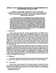
Figure 2: Scheme of learning semantic profiles from a set of image - radiology report pairs. (a) True hidden labeling of the data representing diseases in an organ that coincide with distinct tissue types, blue is healthy tissue. (b) Radiology reports can be used as souce to extract the weak labels. (c) This results in weak labels on the image level are available during training. (d) First, visual appearance is captured by local image descriptors. Then, weak label information is used to remap the local purely visual descriptors to local semantic profiles.
retrieval result. The learning technique is based on randomized subspace partitioning and subsequent analysis of label distributions in the partitions. The feature space partitioning is performed by so called random ferns [19]. An ensemble of such random ferns is used to embody a model of the label distribution in the feature space. During retrieval, this distorts the similarity function so that it is dominated by partitions that are informative for the difference between specific pathologies / classes. The iterative randomized partitioning of a feature space by Random Ferns that we utilize has been used for a fast keypoint recognition technique [18, 19] and as an alternative to k-means clustering for the bag of visual words approach [20, 17], since it offers very fast runtimes.
2.1. Problem definition We are given a set I = {I1 , I2 , ..., II } of I images. For each image, there exists an oversegmentation of Si supervoxel [12] where pi,s identifies the supervoxel s in image PI Ii . We collect all N = ( i=1 Si ) super voxel identifiers N = {p1,1 , . . . , p1,S1 , p2,1 , . . . , pI,1 , . . . , pI,SI } in all I images. We assume that each supervoxel belongs to one of T tissue classes (e.g. ’healthy’,’groundglass’, ...), defining a labeling l : N → {1, . . . , T }. (1) During training this labeling is not given for individual supervoxels. Instead, for each image, we are given a set of labels Ti ⊆ {1, . . . , T } corresponding to an entire image volume. Similar to multi label multi instance learning, for each of these labels, there exists at least one supervoxel in the volume. This results in training data
2. Method hIi , Ti ii=1,...,I , The method consists of a training and an indexing- or application phase. During training (Sec. 2.2) multiple dense, random, independent partitionings of the feature space are generated by a random ferns ensemble [19] (Figure 3 (1)). Based on the label distributions in the resulting partitions, a remapping of feature vectors is generated that captures the link between appearance and weak labels (Figure 3 (2)). In the indexing- or application phase (Sec. 2.3), an ensemble affinity for a novel record to each class is calculated, and a corresponding semantic profile feature vector is generated.
(2)
i.e., for each image we have a set of supervoxels and a set of labels, hPi , Ti i, where ∀t ∈ Ti : ∃pi,s : l(pi,s ) = t.
(3)
To facilitate reading, we define the set Ct of supervoxels across the entire training set associated with a weak label t by this labeling, so that ∀pi,s : (pi,s ∈ Ct )|t ∈ Ti .
(4)
1
unsupervised feature-space partitioning
2
weakly supervised builing of a label distribution model for each class
Figure 3: Label distribution model: (1) Multiple random partitionings of the feature space are generated without supervision. (2) For a certain class, the relative term frequency is calculated. To calculate the ensembles affinity prediction of a novel supervoxel to a class, the K partitions with the highest relative term frequencies are used to indicate a ferns vote. Note that Ct contains many supervoxels that do not carry the true label t. We aim for a similarity measure d that is based on the visual appearance of supervoxels, and at the same time reflects the true labels (that are never directly accessible during training) of two supervoxels. Let a, b, c ∈ N be three supervoxel identifiers. We want to optimize d to come as close to the desired property of: d(a, b) < d(a, c) | l(a) = l(b) ∧ l(a) 6= l(c)
(5)
To this end, we generate a visual descriptor fpSP for each i,s supervoxel, so that the euclidean distance between the descriptors comes close to this aim.
2.2. Linking weak labels and features We are given arbitrary texture descriptors f describing the visual contents of the supervoxels. We learn models of the class label distributions in this primary feature space, and remap each texture descriptors to a new descriptor that is sensitive to the anomaly classes in the weakly labeld training data. Random Subspace Partitioning: We use Random Ferns [18, 19] for space partitioning. A fern F is a sequence of binary decision functions F = hL1 , L2 , . . . , LL i,
(6)
which when applied to a feature vector f result in a binary vector encoding the partitioning of the feature space L(f ) : f 7→ {0, 1}, and
F(f ) : f 7→ {0, 1}L .
(7)
The binary codes represent values in the range (1, . . . , 2L ). We use the binary decision function suggested by Pauly et al. [20]: ( l > 0 if (ssub ) · f subl ≤ τl l Ll (f ) = (8) subl > 1 if (sl ) · f subl > τl
For a split test, a set of dimensions from the feature space is randomly selected and only the corresponding sub vector f subl is considered. The sub vectors are then projected into a one-dimensional space by building the dot product with l unit vector ssub randomly sampled from the unit sphere so l subl > that (sl ) · f subl is a scalar. To get a binary value, this scalar is compared to a threshold τl . We randomly sample this threshold from the projected values. We generate an ensemble E of E Random Ferns of depth L to iteratively partition the feature space. E = hF1 , . . . , FE i
(9)
The ensemble generates E independent partitionings so that E : Rd → {1, . . . , 2L }E (10) E(f ) : f 7→ hy1 , . . . , yE i, y ∈ {1, . . . , 2L }
(11)
We define Yye as the set of supervoxels in a certain partition y of fern Fe so that ∀i ∈ N : i ∈ Yye | Fe (fi ) = y
(12)
Label Distribution Model: For all Yye , we analyse the ratios of the weak labels according to their relative class frequencies. The relative class frequency makes leaf nodes or partitions comparable with respect to the number of examples of a certain class they hold. Some leaf nodes may hold very few or even just a single example. We use Laplace smoothing [3, 21] to diminish an overrating of such small example groups. We define f (Yye , t) as the smoothed relative class frequency of t in the leaf set Yye : f (Yye , t) =
1 + l(Yye , t) PT γ + j=1 l(Yye , tj )
(13)
where γ is a factor to control the impact of the smoothing and l(Yye , t) gives the number of examples in the leaf node Yye that are represented in Ct : l(Yye , t) =
N X
1Yye (i)1Ct (i)
(14)
i=1
The use of f reduces the value of the relative class frequency for small partitions.
2.3. Mapping the features to the classes We define Kt = {he1 , y1 i, . . . , heK , yK i}
(15)
as the set of the K leaf nodes in the ensemble with the K highest values of f (., t) indexed by fern index ei and leaf index yi . Let’s consider a hypothetical supervoxel that is represented in all leaf nodes in Kt . This supervoxel is seen as a prototype representative of class t. Note, that this represents an area rather than a point in the feature space. We interpret the similarity of a supervoxel to this prototype as a measure of its affinity to the class. We construct an affinity indicator for a supervoxel j reflecting its affinity to a class t: E X 2L X dE (j, t) = 1Yye (j)1Kt (he, yi)). (16) e=1 y=1
dE (j, t) sums the occurrences of a supervoxel in Kt so that dE (j, t) ∈ 0, . . . , E. For a supervoxel j, dE (j, t) is calculated for t = 1, . . . , T resulting in a new vector. The maximum possible number of votes from the ensemble for one class is E. In practice, this value will be smaller and vary between different classes. Thus, we scale each dimension to [0, 1] resulting in the new feature vector for each supervoxel that we call semantic profile (SP): fjSP ∈ [0, 1]T = [dE (j, 1), . . . , dE (j, T )]]
(17)
We expect that this descriptor provides a higher specificity in retrieving representatives of the learned anomaly classes compared to a feature vector resulting from a descriptor that is learned on visual information only.
3. Evaluation We evaluated two aspects of semantic profiles: (1) do they improve retrieval accuracy in clinical imaging data, and (2) do they map terms in radiology reports accurately to regions in the corresponding imaging data? We want to understand if injecting weak label information can improve retrieval over purely visual features, and if the corresponding descriptors indicate a mapping of terms to the individual volumes.
Data We performed experiments on a set of 300 high resolution computed tomography (HRCT) scans of lungs provided by LTRC [11]. All voxels in the images are labelled into one of five tissue classes: healthy lung texture and four tissue types (ground-glass, reticular pattern, honey combing, emphysema) occuring in interstitial lung diseases (ILD). Only voxels within the lungs are analyzed. We transform all volumes to an isotropoic voxel resolution of 0.7mm3 in advance, and perform over-segmentation of the volumes to monoSLIC supervoxels of an average size of 1cm3 [12]. We consider only supervoxels consisting of at least 70% of one label, to avoid partial volume effects. For the experimental validation we created a weakly labeled data set from the labeled lung data. To simulate a varied distribution of labels in the training dataset we sample 683201 supervoxels of which 460912 show healthy, 42183 show ground-glass, 7461 show reticular, 12436 show honeycombing and 160980 show emphysema. The sets Ct are bagged to create a set equivalent to what would be training data from a clinical source for the proposed algorithm. Only the set membership C1 ..C5 is known to the learning algorithm. Since their distribution is relevant we show it in Table 1. The negative instances in each bag are chosen to represent in extent 10% of the population of the other classes. Healthy lung texture is a special case as it can be expected to be present in every lung. In a real world setting, additional control examples of healthy lung texture can be sampled from records of healthy lungs. Thus, a set of healthy representatives C1 can be obtained. All experiments are performed by 10-fold crossvalidation. The splitting into training and testset is performed under consideration of the original volume membership of the supervoxels into 30 test and 270 training volumes in order to prevent any wihtin-patient overlap between training and test set. We extract two texture descriptors for each supervoxel. (1) 1200-dimensional Texture Bags [4], a multi-scale Bag of Visual Words (BVW) approach on Local Binary Patterns (in the following abbreviated with BVW), and (2) 52-dimensional Haralick features [10] on 21 × 21 × 21 patches around the center of the supervoxel. Both methods have been used for retrieval of anomalies in lung CTs [4, 14, 25, 6]. For each descriptor, we generate a semantic profile mapping. We term the novel features SP-BVW and SP-Haralick for the respective embedding into the 5dimensional (5 indicators for healthy and the 4 anomalies) feature space. For all experiments we fixed the parameters for number of ferns E = 1000 and fern depth L = 8. Retrieval To evaluate retrieval we randomly choose 200 supervoxels of each anomaly class from the testset as queries (overall 1000 queries). Based on each query, we rank the training data using Euclidean distance among 4 feature vectors: (1) BVW, (2) Haralick, (3) SP-BVW, and (4) SP-
Anomaly name Healthy Ground-glass Reticular Honeycombing Emphysema
Class t= 1 2 3 4 5
# Healthy 276547 46091 46091 46091 46091
# Ground-glass 0 41682 4138 4138 4138
# Reticular 0 746 7464 746 746
# Honeycombing 0 1246 1246 12463 1246
# Emphysema 0 16098 16098 16098 160980
Σ 276547 105563 75037 79536 213201
TP in % 100 40 10 13 76
Table 1: Composition of the sets C1 to C5 . Each line shows the distribution of the true classes in one set. The sum of supervoxels Σ in each set and the share of True Positive representatives (TP) are shown on the right. During learning, only the set (C1 to C5 ) memberships but not the true classes are visible to the training algorithm. 0.7 0.6
average MAP
0.5 0.4 0.3 0.2 SP−BVW
0.1 0 1 10
SP−Haralick 2
10
3
10 K
4
10
5
10
Figure 4: Effect of parameter K on the retrieval performance. The plot shows the averaged MAP over the five classes for values of K from 10 to 105 . Haralick. We compare recall and precision achieved by these descriptors. Mapping terms to images We map the individual coefficients of the semantic profiles back to the volume to evaluate if they allow for localization of the tissue areas responsible for specific retrieval. We evaluate this qualitatively (Figure 6) and quantitatively (Table 3), by classifying supervoxels based on the highest coefficent of the corresponding semantic profile. Note that this is not a sophisticated classifier, but an inspection if the features capture the actual tissue properties accurately. These experiments are performed on volumes of the test set.
4. Results Retrieval Figure 5 shows precision-recall curves for the five tissue classes. Baseline, i.e., random-ranking is indicated by a gray line. Table 2 lists the corresponding mean average precision values (MAP). Semantic profiles return better precision for all anomaly classes in comparison to the corresponding purely visual descriptors. A distinctive improvement can be seen from BVW to SP-BVW for the retrieval of ground-glass supervoxels (MAP of 0.22 to 0.71). Comparing the visual descriptors to the semantic profile embedding
the averaged MAP over the five classes is raised from 0.38 to 0.58 for BVW and from 0.53 to 0.65 for Haralick. Figure 4 shows the effect of the parameter K on the retrieval performance. If K is chosen too low, the model of the label distribution in the feature space is too sparse, if K is chosen too high the model associates regions in the feature space that have no association to the modelled class. Figure 7 shows examples of queries and resulting nearest neighbor supervoxels using BVW and SP-BVW descriptors. One can see the suppression of the (for this anomaly irrelevant) rotation variant features of the BVW descriptor resulting from re-mapping to semantic profiles. Mapping terms to images Figure 6 shows ground truth labelings of volume data, and a labeling obtained by assuming that the highest semantic profile coefficient is a good estimator for the correct label. Corresponding quantitative results for the best performing descriptor (SP-Haralick) are shown in Table 3. The right side of Figure 6 shows the mapping of the semantic profiles back to the imaging data. Note how the distribution of voxel scores learned from weakly labeled volumes, mirrors the true voxel labels very well. Runtime To generate E = 1000 partitionings, runtime for the unsupervised part of the training (Figure 3 (1)) on 615000 52-dimensional Haralick features is 85 seconds. The iterative modeling of the label distribution in the feature space (Figure 3 (2)) needs 20 seconds per class (100 seconds for 5 classes). This runtime experiments have been performed on a 12-core 24 thread Intel Xeon processor utilizing a Matlab implementation of the method. The calculation of the semantic profiles for 7526 haralick descriptors (average number of supervoxels for a volume) needs 1.37 seconds.
5. Conclusion In this paper we propose and evaluate semantic profiles that capture visual information related to clinically relevant terms. Training of semantic profiles is weakly supervised. It is based on pairs of image volumes and corresponding sets of terms in radiology reports that describe radiological findings present in the imaging data. We show that the resulting descriptor substantially improves retrieval precision and re-
Table 2: MAP in % for retrieval of four anomaly classes and healthy. Semantic Profile embedding increases the MAP significantly over the visual descriptors used as input for the learning algorithm. Best MAP for each class is marked bold.
Figure 6: Left: Mapping terms to the volume data. Ground truth labeling not available during training and the label of highest semantic profile coefficient for the same image slice. Right: maps of the semantic profiles used for retrieval mapped back to the data. Red indicates high values for a pathology pattern, blue indicates low values.
114922 227 80 471 2247 0.99 0.86
459 3789 266 20 0 0.92 0.99
35 116 381 22 1 0.51 1.00
353 2 16 717 36 0.57 1.00
34 0 0 2 13811 0.86 1.00
Table 3: Confusion Matrix and Sensitivity and Specificity values for supervoxel labeling on the basis of the highest semantic profile coefficient on SP-Haralick
References call. Furthermore it allows to map terms back to regions in the imaging data. The method improves retrieval in medical imaging data since it augments the representation of image characteristics that are linked to diagnostically relevant terms. Importantly, it can be trained based on data generated during clinical routine, without the need for additional annotation.
[1] S. Andrews, T. Hofmann, and I. Tsochantaridis. Multiple instance learning with generalized support vector machines. In AAAI/IAAI, pages 943–944, 2002. [2] T. L. Berg, A. C. Berg, and J. Shih. Automatic attribute discovery and characterization from noisy web data. In Computer Vision–ECCV 2010, pages 663–676. Springer, 2010. [3] H. Bostrom. Estimating class probabilities in random forests.
1
Healthy
1
0.9
0.9
0.8
0.8
0.7
0.7
0.6
0.6
0.5
0.5
0.4
0.4
0.3
0.3
0.2
0.2 0.1
0.1 0 0
0.1 0.2 0.3 0.4 0.5 0.6 0.7 0.8 0.9
1
Reticular
0.9
1
0 0 1 0.9
0.8
0.8
0.7
0.7
0.6
0.6
0.5
0.5
0.4
0.4
0.3
0.3
0.2
0.2
0.1
0.1
0 0 1
Ground-glass
0.1 0.2 0.3 0.4 0.5 0.6 0.7 0.8 0.9
1
Emphysema
0 0
0.1 0.2 0.3 0.4 0.5 0.6 0.7 0.8 0.9
1
Honeycombing
0.1 0.2 0.3 0.4 0.5 0.6 0.7 0.8 0.9
(a)
1
BVW SP−BVW Haralick SP−Haralick baseline
0.9 0.8 0.7 0.6 0.5 0.4 0.3 0.2 0.1 0 0
0.1 0.2 0.3 0.4 0.5 0.6 0.7 0.8 0.9
(b)
Figure 7: Nearest neighbors for four different query supervoxels (red box) using (a) BVW descriptor and (b) the Semantic Profiles trained on BVW.
1
Figure 5: Precision Recall curves for the four anomaly classes and healthy. Comparison of the texture descriptors BVW and Haralick and the Semantic Profile embeddings of both.
In Sixth International Conference on Machine Learning and Applications, pages 211–216. IEEE, 2007. [4] A. Burner, R. Donner, M. Mayerhoefer, M. Holzer, F. Kainberger, and G. Langs. Texture bags: anomaly retrieval in medical images based on local 3d-texture similarity. In Medical Content-Based Retrieval for Clinical Decision Support, pages 116–127. Springer, 2012. [5] J. Dash, R. Gupta, S. Mukhopadhyay, N. Khandelwal, P. Bhattacharya, and M. Garg. Content-based image retrieval for interstitial lung diseases. In Signal Processing, Computing and Control (ISPCC), 2012 IEEE International Conference on, pages 1–4, March 2012. [6] A. Depeursinge. Affine–invariant texture analysis and retrieval of 3D medical images with clinical context integration. PhD thesis, University of Geneva, 2010. [7] A. Depeursinge, D. Van de Ville, A. Platon, A. Geissbuhler, P.-A. Poletti, and H. Muller. Near-affine-invariant texture learning for lung tissue analysis using isotropic wavelet frames. Information Technology in Biomedicine, IEEE Transactions on, 16(4):665–675, 2012. [8] J. G. Dy, C. E. Brodley, A. Kak, L. S. Broderick, and A. M. Aisen. Unsupervised feature selection applied to content-
based retrieval of lung images. IEEE Transactions on Pattern Analysis and Machine Intelligence, 25(3):373–378, 2003. [9] M. Guillaumin, J. Verbeek, and C. Schmid. Multiple instance metric learning from automatically labeled bags of faces. In Computer Vision–ECCV 2010, pages 634–647. Springer, 2010. [10] R. M. Haralick. Statistical and structural approaches to texture. Proceedings of the IEEE, 67(5):786–804, 1979. [11] D. Holmes III, B. Bartholmai, R. Karwoski, V. Zavaletta, and R. Robb. The lung tissue research consortium: an extensive open database containing histological, clinical, and radiological data to study chronic lung disease. In The Insight Journal, 2006 MICCAI Open Science Workshop, pages 1–5, 2006. [12] M. Holzer and R. Donner. Over-segmentation of 3d medical image volumes based on monogenic cues. In Proceedings of the 19th CVWW, pages 35–42, 2014. [13] R. Jin, S. Wang, and Z.-H. Zhou. Learning a distance metric from multi-instance multi-label data. In IEEE Conference on Computer Vision and Pattern Recognition, CVPR 2009., pages 896–902. IEEE, 2009. [14] M. Lam, T. Disney, M. Pham, D. Raicu, J. Furst, and R. Susomboon. Content-based image retrieval for pulmonary computed tomography nodule images. In Medical Imaging, pages 65160N–65160N. International Society for Optics and Photonics, 2007. [15] C. P. Langlotz. Radlex: A new method for indexing online educational materials 1. Radiographics, 26(6):1595–1597, 2006.
[16] C. Leistner, A. Saffari, and H. Bischof. Miforests: Multipleinstance learning with randomized trees. In Computer Vision–ECCV 2010, pages 29–42. Springer, 2010. [17] Y. Mu, J. Sun, T. X. Han, L.-F. Cheong, and S. Yan. Randomized locality sensitive vocabularies for bag-of-features model. In Computer Vision–ECCV 2010, pages 748–761. Springer, 2010. [18] M. Ozuysal, M. Calonder, V. Lepetit, and P. Fua. Fast keypoint recognition using random ferns. IEEE Transactions on Pattern Analysis and Machine Intelligence, 32(3):448–461, 2010. [19] M. Ozuysal, P. Fua, and V. Lepetit. Fast keypoint recognition in ten lines of code. In Conference on Computer Vision and Pattern Recognition, CVPR 2007., pages 1–8. IEEE, 2007. [20] O. Pauly, D. Mateus, and N. Navab. Building implicit dictionaries based on extreme random clustering for modality recognition. In Medical Content-Based Retrieval for Clinical Decision Support, pages 47–57. Springer, 2012. [21] F. Provost and P. Domingos. Tree induction for probabilitybased ranking. Machine Learning, 52(3):199–215, 2003. [22] G.-J. Qi, X.-S. Hua, Y. Rui, T. Mei, J. Tang, and H.-J. Zhang. Concurrent multiple instance learning for image categorization. In IEEE Conference on Computer Vision and Pattern Recognition, CVPR’07., pages 1–8. IEEE, 2007. [23] J. Shotton, M. Johnson, and R. Cipolla. Semantic texton forests for image categorization and segmentation. In IEEE Conference on Computer Vision and Pattern Recognition, CVPR 2008., pages 1–8. IEEE, 2008. [24] A. Smeulders, M. Worring, S. Santini, A. Gupta, and R. Jain. Content-based image retrieval at the end of the early years. IEEE Transactions on Pattern Analysis and Machine Intelligence, 22(12):1349–1380, 2000. [25] Y. Xu, M. Sonka, G. McLennan, J. Guo, and E. A. Hoffman. Mdct-based 3-d texture classification of emphysema and early smoking related lung pathologies. IEEE Transactions on Medical Imaging, 25(4):464–475, 2006. [26] Z.-J. Zha, X.-S. Hua, T. Mei, J. Wang, G.-J. Qi, and Z. Wang. Joint multi-label multi-instance learning for image classification. In IEEE Conference on Computer Vision and Pattern Recognition, pages 1–8. IEEE, 2008.