MASTER-SLAVE SYNCHRONIZATION OF ROBOT

MASTER-SLAVE SYNCHRONIZATION OF ROBOT MANIPULATORS: EXPERIMENTAL RESULTS Anne Karin Bondhus ∗ Kristin Y. Pettersen ∗ Henk Nijmeijer ∗∗ ∗ Department of Engineering Cybernetics, Norwegian University of Science and Technology, N-7491 Trondheim, Norway ∗∗ Department of Mechanical Engineering, Eindhoven University of Technology, PO Box 513, 5600 MB Eindhoven, Netherlands

Abstract: This paper presents experimental results for master-slave synchronization of two robot manipulators using a recently developed observer-controller scheme. The paper aims to investigate the value and the limitations of the theory. In particular, the theoretical result of uniform ultimate boundedness of the synchronization errors is investigated. Back-to-back simulation results are also c presented. Copyright °2005 IFAC Keywords: Synchronization, Robot manipulators, Observers, Experimental results, Ultimate boundedness

1. INTRODUCTION

the theory. The back-to-back simulations are also presented for comparison.

In (Bondhus et al., 2004) we presented a new method for master-slave synchronization of mechanical systems, with no force feedback. This method can be used in a teleoperation system when the task of the slave system is to track the measured trajectory of a mechanism moved by a human operator. The master-slave synchronization can also be applied to problems where two systems are to follow the same trajectory given mathematically; only with a constant offset between the trajectories. An example is two vehicles (ships, cars, mobile robots etc.) that are to move in a synchronized manner.

The type of problem considered in Bondhus et al. (2004) and in this work is similar to the problems studied in Rodriguez-Angeles (2002)/Nijmeijer and Rodriguez-Angeles (2003). Both in Bondhus et al. (2004) and in Nijmeijer and RodriguezAngeles (2003) a master-slave synchronization scheme was developed based on the use of observers to estimate the velocities. The experimental results and simulation results in this paper show that our method has similar performance to the method in Nijmeijer and RodriguezAngeles (2003). However, because we use small gain arguments in the theoretical analysis instead of a Lyapunov function for the total system as in Nijmeijer and Rodriguez-Angeles (2003), the analysis in (Bondhus et al., 2004) give simpler theoretical expressions for the transient bounds and ultimate bounds of the synchronization errors

In this paper we will present the experimental results for the synchronization scheme in Bondhus et al. (2004) applied to master-slave synchronization of two robots. The aim is to obtain a better understanding of the value and the limitations of

and observer errors. This makes the gain tuning easier. In addition the choice of observers is more flexible, because the theoretical analysis based on the small gain theorem will be similar for all types of observers, as long as the observers have been shown to satisfy certain requirements.

g(x1 ) ∈ Rn is the vector of generalized gravitational forces and f (x2 , θ) is the friction term. The inertia matrix is known to be symmetric and positive definite. Among the model parameters only the friction parameters are assumed to be uncertain.

This paper is organized as follows. In Section 2 the models are described, and Section 3 presents the general form of the observers in the synchronization scheme, together with the observers used in the experiments and simulations in this work. In Section 4 the control input is presented. Section 5 describes the experimental setup, while Section 6 presents and discusses the experimental and simulation results.

The friction term f (x2 , θ) is modelled by the same model as in Nijmeijer and Rodriguez-Angeles (2003), which is a special case of the friction model in Hensen et al. (2000). The friction in joint j is fj and it is only dependent on the velocity x2j of joint j. The model is ¶ µ 2 fj (x2j , θ) = Bvj x2j + Bf 1j 1 − 1 + e2w1j x2j µ ¶ 2 + Bf 2j 1 − (4) 1 + e2w2j x2j

2. THE ROBOT MODELS

where Bvj x2j is the viscous friction and the remaining terms model the Coulomb and Stribeck friction.

We consider the problem of master-slave synchronization of two robots, which we assume to be fully actuated. It is assumed that the robots have the same geometry in the sense that they have the same type of joints, although the physical parameters like masses, inertia and lengths of the links may be different. Only the joint positions of the robots are measured. The objective is that the joint positions of the slave robot should track the measured joint positions of the master robot. The master robot is controlled independently of the movement of the slave robot. For the master robot any conventional controller can be used for tracking the desired trajectory. For the slave robot a model-based observer will be included in the synchronization scheme, and therefore a mathematical model of the slave robot is needed. For the master robot a mathematical model is not essential for the synchronization scheme. If a physically based model of the master robot is not known, the trajectory of the master robot can be modelled, for instance, by a set of double ¨ m , where the integrators: x˙ 1m = x2m , x˙ 2m = q ¨ m is an unknown input. acceleration q The model of the slave robot can be written as x˙ 1 = x2

(1) −1

x˙ 2 = M

(x1 )τ + β(x1 , x2 , θ)

(2)

with β(x1 , x2 , θ) = M−1 (x1 ) [−C(x1 , x2 )x2 − g(x1 )] − M−1 (x1 )f (x2 , θ)

(3)

3. THE ROBOT OBSERVERS This section presents the observers used in the experiments and simulations in this paper. General expressions for the observers are also given, as the control in Section 4 is expressed in terms of general observer terms. For the slave robot the observer developed in Berghuis and Nijmeijer (1993) and Berghuis (1993) was used. We extend the observer by including a term to account for the friction model. The observer is then given by ˆ˙ 1 = g1 (x1 , x ˆ1, x ˆ2) x (5) ˆ (6) ˆ˙ 2 = M−1 ˆ1, x ˆ 2 )τs + g2 (x1 , x ˆ1, x ˆ 2 , θ) x o (x1 , x with Mo = M(x1 ) and ˆ1, x ˆ2) = x ˆ 2 + Ld x ˜1 g1 (x1 , x ˆ1, x ˆ 2 ) = −M g2 (x1 , x −1

+M

−1

(7)

ˆ + Lp2 x ˜1 (x1 )f (ˆ x2 , θ)

˜1) (x1 ) (−C(x1 , q˙ 0 )q˙ 0 − g(x1 ) + Lp1 x (8)

˜ 1 := x1 − x ˆ 1 and The observer errors are x ˜ 2 := x2 − x ˆ 2 , and we let x ˜ := [˜ ˜ T2 ]T . The x xT1 , x variable q˙ 0 is defined by ˆ˙ 1 − Λ2 x ˜1 = x ˆ 2 + (Ld − Λ2 )˜ q˙ 0 = x x1 (9) with Λ2 = ΛT2 > 0. The gain matrices in the observer should satisfy Ld = LTd > 0, Lp1 = LTp1 > 0, Lp2 = LTp2 > 0. The gain matrices are also assumed to satisfy the following assumption:

p

where θ ∈ R is a vector of the p parameters in the friction model. The vector x1 ∈ Rn is the vector of generalized coordinates (joint positions/orientations) and the vector x2 ∈ Rn is the vector of generalized velocities. The vector τs ∈ Rn is the generalized joint forces, M(x1 ) ∈ Rn×n is the inertia matrix, C(x1 , x2 )x2 ∈ Rn is the vector of generalized centripetal and Coriolis forces,

Assumption 1. Ld , Lp1 , Lp2 and Λ2 are constant and diagonal. Moreover, Ld and Lp2 can be written as Ld = ld I + Λ2 and Lp2 = ld Λ2 . For the master robot we may also use an observer based on a physical model of the robot, but to investigate the synchronization scheme performance

when a master model is not available we have in this paper applied the high gain observer of Dabroom and Khalil (1997) for the master trajectory. For this observer the the master robot is just modelled as a double integrator as described in Section 2.

5. EXPERIMENTAL SETUP

The high gain observer is given by ˆ˙ 1m = g3 (x1m , x ˆ 1m , x ˆ 2m ) x ˙x ˆ 2m = g4 (x1m , x ˆ 1m , x ˆ 2m )

(10) (11)

with ˆ 2m + D1 x ˜ 1m , g3 = x

˜ 1m g4 = D2 x

(12)

˜ 1m := x1m − x ˆ 1m , where the observer errors are x ˜ 2m := x2m − x ˆ 2m , and we let x ˜m ³ ˜ T2m ]T´. x = [˜ xT1m , x α α The gain matrices are D1 = diag ²1,1 , · · · ²1,n 1 n ³ ´ α2,1 α2,n and D2 = diag ²2 , · · · ²2 . In Dabroom and n 1 Khalil (1997) it was shown that the high gain ˆ 2m is equivalent to the output found estimate x by running x1m through a second order filter in series with a differentiator. The synchronization scheme developed in Bondhus et al. (2004) was developed for observers in the general form given by (5-6) and (10-11), with g1 , g2 , g3 and g4 locally Lipschitz, and Mo nonsingular.

4. THE CONTROLLER In the experiments in this paper we have applied the control deduced in (Bondhus et al., 2004), which is given by τs = Mo {fs (s) − g2 + g4 − Λ(g1 − g3 )}

(13)

with ˆ 2m ) + Λ(ˆ ˆ 1m ) s = (ˆ x2 − x x1 − x

(14)

where Λ is a positive definite matrix. The choice of f (s) must be such that the dynamics s˙ = fs (s) are globally asymptotically stable. We have here used fs (s) = −As s, where As is diagonal and positive definite. The functions g1 , g2 , g3 and g4 are in this paper the observer terms given by (7-8) and (12). The theoretical result of uniform ultimate boundedness of the synchronization errors requires that the combination of the dynamics of the synchronization errors and the dynamics of the observer errors must satisfy the requirements given in Bondhus et al. (2004, Th. 1). The dynamics of the synchronization position error can be found from the definition of s in (14) as shown in Bondhus et al. (2004). The analysis to show that the specific slave observer used in the experiments in this paper satisfy the conditions needed in Bondhus et al. (2004, Th. 1) are presented in (Bondhus, 2004).

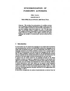
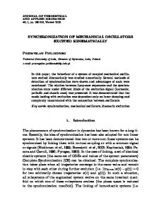
Fig. 1. The industrial transposer robot R1 used in the synchronization experiments Experiments and simulations were performed for the synchronization of two industrial transposer robots designed by the Centre for Manufacturing Technology (CFT) Philips laboratory. One of the robots is shown in Fig. 1. The other robot is of the same type and size, and it has the same geometric parameters such as lengths of the links. The robots are installed at the Dynamics and Control Technology Laboratory at the Eindhoven University of Technology. They are fully actuated by brushless DC servomotors. Although the shaft of the motors and the corresponding links are connected by belts, the pair servomotor-link proved to be stiff enough to be considered a rigid joint. For implementation of the controllers and communication with the robots, the experimental setup is equipped with a DS1005 dSPACE system, with a processor PPC750, a 480 MHz clock and an 80 MHz bus clock. Throughout the experiments the sampling frequency of the DS1005 dSPACE system was 2kHz. The robot models are described in Nijmeijer and Rodriguez-Angeles (2003, App. H) and in more detail in Rodriguez-Angeles et al. (2002). The master robot is the one designated as Robot 1 (R1) and the slave robot is the one designated as Robot 2 (R2). We will now give a summary of the most important aspects of the models. The robots have four degrees of freedom and seven joints. The four Cartesian degrees of freedom are denoted by xc1 , xc2 , xc3 and xc4 . The variables xc1 and xc2 denote up/down and forward/backward movement of the arm respectively, and xc3 , xc4 are the rotation and translation of the base on which the arm is mounted. The coordinates xc3 and xc4 are absolute coordinates and are referred to with respect to an inertial frame, frame {0}, at the base of the robot. Meanwhile xc1 , xc2 are relative coordinates and are referred to with respect to a frame at the edge of the translational platform, frame {e}. The upper arm has a pantographic design as shown in Fig. 2. The motors give forces

performed under ideal conditions, i. e. with a perfect friction model, perfect system model and without measurement noise.

P4

L6

P3

α

xcj,d (t) = a0,j + a1,j sin(2sfj πωt) + a2,j sin 4sf,j πωt + a3,j sin(6sf,j πωt) + a4,j sin(8sf,j πωt) (21)

P2 L4

β

y

r

P1 xr

x 0’ 0.1 m

Fig. 2. The pantographic design of the upper arm along the axes xr and yr . The values of xr and yr determine the values of the two angles α and β shown in Fig. 2. The relation between xr , yr and α, β is given by −xr r β = arccos + arccos (15) r 2L4 and  ³ ´  arcsin yr − sin(β) ³ L4 ´ (16) α=  arccos −xr − cos(β) L4 with r = x2r + yr2 , and L4 a geometric parameter shown in Fig. 2. The measured variables are xr , yr , xc3 and xc4 . Between the variables xr , yr and respectively xc1 , xc2 there are kinematic relations involving only these variables and the geometric parameters of the robot, i. e. xr = xr (xc2 , θR ) and yr = yr (xc2 , θR ) where θR contains the geometric parameters of the robot.

Table 1. Desired trajectory parameters.(j=2, 3, 4 [m], j=3 [rad]) ai,j j=1 j=2 j=3 j=4

i=0 -0.1343 0.2766 2.4 -0.265

i=1 -0.05 0.05 0.15 0.2

(17) (18) (19) (20)

with ds = 0.185. We see that q1 is a linear distance, while q2 , q4 and q5 are angles. We add the index m for the master, and s for the slave. With the notation used in the earlier sections x1m = [q1m , q2m , q4m , q5m ]T and x1 = [q1s , q2s , q4s , q5s ]T . Both robots have the same inverse kinematics from the Cartesian coordinates to the joint coordinates as given by Equations (17-20). 6. RESULTS This section presents the experimental results for the synchronization of the robots described in Section 5, using the master-slave synchronization scheme presented in Sections 3-4. The aim is to better understand the relation between theory and practice. To this end we also provide a backto-back comparison with simulations, that were

i=2 -0.015 0.03 0.05 0.1

i=3 -0.005 -0.03 -0.03 -0.05

i=4 -0.01 0.02 0.02 0.05

The desired trajectory was transformed by the kinematic equations to a desired trajectory in the joint coordinates. Fig. 3 shows the desired trajectory in the joint space. In the simulations a model 0.1 0.2 0 −0.1

0.1 0

−0.1 −0.2

−0.2

0

5

10 time [s]

15

−0.8

−1

2

4 time [s]

6

2

4 time [s]

6

2

1.9

−1.1 0

0

2.1

−0.9

The joint coordinates are defined by q1 := xc4 + ds π q2 := xc3 − − 0.8292 2 π q4 := −β + 2 q5 := β − α

with sf,j = 1 for xc1 , xc2 and xc3 , and sf,j = 0.25 for xc4 , and the other parameters given in Table 1

q2 [rad]

L5

q5 [rad]

P5

The desired trajectory of the master robot was given in Cartesian coordinates by

L6

q1 [m]

L4

β

0’

q4 [rad]

y

2

4 time [s]

6

1.8 0

Fig. 3. Desired trajectory (xd ) for the master robot of the master robot was not included as the ability of this robot to follow its reference trajectory is not of central importance. The important feature of the synchronization scheme is the ability of the slave manipulator to follow the actual behaviour of the master robot. Therefore, to get a better comparison between theory and experiments with respect to this main feature, we used the measured trajectory of the master robot in the experiment as master trajectory in the simulations. This implies that the master trajectory to be followed by the slave robot was the same in the simulations as in the experiments. A friction model was included in the observer of the slave robot as described by (4-8). We have used the estimates of the friction parameters found in Rodriguez-Angeles et al. (2002), although these parameters were not expected to be very accurate since the friction changes with time

and temperature. The friction parameters are presented in Table 2. In the simulations these friction Table 2. Friction parameters.(j=1 [N], j=2, 3, 4 [Nm]) Joint q1 q2 q4 q5

Bvj 97.2600 9.0999 11.6257 9.6229

Bf 1,j Bf 2,j w1,j w2,j -54.9912 -46.5915 150.3190 -98.9881 18.4710 11.1605 136.8945 -170.4702 -3.5232 2.2684 -35.3699 -89.3236 -5.8564 8.2304 36.0641 16.2942

parameters were used both in the simulation of the robot dynamics and in the observer, i. e. the simulations were performed under the ideal condition of a perfect friction model. An experiment was also performed with a 30 % reduction in all the friction parameters. The master robot was controlled by PD-controllers in the Cartesian space. These simple controllers were used for the master robot, as the objective of this work was to investigate the synchronization scheme, not how well the master robot followed its desired trajectory. For the slave robot the observer given in (5-9) was used, with Lp1 = 100I, Λ2 = 5I, ld = 1000, where I is the identity matrix. The controller matrices in (13) with fs (s) = −As s were chosen as As = 10I and Λ = 100I. For the master robot the high gain observer given by (10-12) was used with α1,i = 16, α2,i = 1 and ²i = 0.01 for i = 1 · · · 4. The gains were chosen through simulations with different gains, aiming at finding gains which gave acceptably small synchronization errors and at the same time control inputs which did not reach the saturation limits. A wide range of gains were seen to give acceptable results. The theoretical conditions the gains must satisfy are presented in (Bondhus, 2004). Although the deduction of these conditions is long, the conditions themselves are quite simple. However, the conditions are conservative. In the simulations and in practice the synchronization was seen to work with much lower gains than required by the theoretical conditions. The gains used here do not satisfy all the theoretical conditions. The initial values are shown in Table 3. Here x1d is the desired position of the master robot, and x2d the desired velocity of the master robot. The other variables are defined earlier in this paper. The initial conditions in the simulations were chosen equal to those in the experiment, except that x1d and x2d were not used, as discussed earlier. Before the start of the synchronization scheme the robots were moved to their initial positions by simple PID-controllers based on filtering of the position measurements. These positions were held for some time and therefore the initial velocities are approximately 0. The initial positions and velocities were the same for both robots due to the original setup of the laboratory, and therefore the synchronization errors were 0 at the start of

Table 3. Initial values for the trajectories and the observers (1) [m] (2) [rad] (3) [rad] x1d -0.08 0 -0.9899 x2d 0.1131 0.8473 -0.1275 x1m -0.08 0 -0.9899 x2m 0 0 0 x1 -0.0797 -0.00027 -0.9848 x2 0 0 0 ˆ 1m -0.08 x 0 -0.9899 ˆ 2m x 0 0 0 ˆ 1 -0.0797 -0.00027 -0.9848 x ˆ2 x 0 0 0

(4) [rad] 1.98045 -0.8749 1.98045 0 2.0035 0 1.98 0 2.0035 0

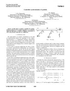
the synchronization. The point t = 0 in the plots in this paper is the time that the synchronization starts. The transient response is small since we had the initial tracking errors and observer errors approximately equal to 0. Fig. 4 shows the timeevolution of the position synchronization errors. We see that the errors do not go to zero. This complies with the theoretical result of uniform ultimate boundedness. The bounds are small although we have not used an accurate friction model. It is also seen from Fig. 4 that reducing all the estimated friction parameters by 30 % does not result in much change in the synchronization errors. This indicates that the synchronization scheme has some robustness with regard to errors in the estimated friction parameters. There are some differences between the simulation results and the experimental results. This is as expected, since the simulation is done under the assumption of a perfect model, exactly known kinematic transformations, no actuator dynamics and no measurement noise. It was seen in the experiment that increasing Λm (The lowest eigenvalue of Λ) gave lower synchronization errors. However, in the experiment there was a limit to the obtainable accuracy because of the resolution of the encoders used to measure the positions, and because the control inputs reached their saturation limits if Λm was too high. The encoder resolution gives an accuracy of ±0.5[mm] in the measured values of xr , yr and xc4 (Nijmeijer and Rodriguez-Angeles, 2003, p.114). Although increasing Λm gives smaller synchronization errors, one must be careful not to increase Λm too much. Increasing Λm gives a higher bound for ||e2 ||∞ , and this may lead to violation of the small gain stability conditions, see Bondhus et al. (2004). Fig. 5 shows the experimental results with the same conditions as before, but with a weight of 2.8 kg placed on the end effector of the slave robot. This does not result in much change in the synchronization errors. There are some spikes that are much higher than before, at about 6.5 s in Fig. 5. From this we see that the synchronization

parameters. This is in accordance with the theory presented in Bondhus et al. (2004). The robustness with regard to modelling errors was investigated experimentally by placing a load on the slave robot. This only resulted in a small change in the synchronization errors, which indicates that the synchronization scheme is quite robust with regard to modelling errors. A full stability analysis was not included because of space limitations, but is given in (Bondhus, 2004).

−3

x 10

1

0.01 e1(2) [rad]

e1(1) [m]

0.5 0

−0.5 −1

−0.01

−1.5 0

5

10 time[s]

15

0

2

4 time[s]

6

0.06 e1(4) [rad]

0.01 e1(3) [rad]

0

0

−0.01 −0.02 0

2

4 time[s]

0.04 0.02

REFERENCES

0

−0.02 0

6

2

4 time[s]

6

Fig. 4. Synchronization errors between measured slave trajectory and measured master trajectory, e1 = x1 −x1m . Experiment with nominal friction parameters (-), Experiment with 30 % reduction in estimated friction parameters (-.-.), Simulation with nominal friction parameters (· · · ) −3

1

x 10

0.01 e (2) [rad]

e1(1) [m]

0.5 0

0

1

−0.5 −1

−0.01

−1.5 0

5

10 time[s]

15

0

e (4) [rad]

e1(3) [rad]

4 time[s]

6

2

4 time[s]

6

0.06

0.01 0

0.04 0.02

1

−0.01 −0.02 0

2

2

4 time[s]

6

0 −0.02 0

Fig. 5. Experimental results with a weight of 2.8 kg on the slave robot scheme is also quite robust with regard to modelling errors.

7. CONCLUSION In this paper we have presented simulations and experimental results for an observer-controller scheme for master-slave synchronization, which was developed in (Bondhus et al., 2004). The bounds for the synchronization position errors in the experiments were seen to be small even though the estimated friction parameters were not very accurate. A reduction of 30% in the nominal friction parameters only resulted in a small change in the experimental synchronization errors. The results indicate that the synchronization scheme is robust with regard to errors in the friction

Berghuis, H. and H. Nijmeijer (1993). A passivity approach to controller-observer design for robots. IEEE Transactions on Robotics and Automation 9(6), 740–754. Berghuis, Harry (1993). Model-based Robot Control: from Theory to Practice. PhD thesis. University of Twente, Netherlands. Bondhus, A. K. (2004). Analysis of a masterslave synchronization scheme using a passivity based slave observer. Technical report 2004-7-w. Norwegian University of Science and Technology, Dept. of Engineering Cybernetics. O. S. Bragstads Plass 2D, 7491 Trondheim. Bondhus, A. K., K. Y. Pettersen and H. Nijmeijer (2004). Master-slave synchronization of robot manipulators. IFAC Symposium NOLCOS 2004, Symposium on Nonlinear Control Systems. Dabroom, A. and H. K. Khalil (1997). Numerical differentiation using high-gain observers. Proceedings of the 36th Conference on Decision & Control, San Diego, California USA. Hensen, R. H. A., G. Z. Angelis, M. J. G. van de Molengraft, A.G. de Jager and J. J. Kok (2000). Grey-box modeling of friction: An experimental case-study. European Journal of Control 6, 258–267. Nijmeijer, H. and A. Rodriguez-Angeles (2003). Synchronization of mechanical systems. World scientific series on nonlinear science. World Scientific Publishing Co. Pte. Ltd. Rodriguez-Angeles, A. (2002). Synchronization of Mechanical Systems. PhD thesis. Technische Universiteit Eindhoven, Netherlands. Rodriguez-Angeles, A., D. Lizarraga, H. Nijmeijer and H. A. van Essen (2002). Modelling and identification of the cft- transposer robot. Technical report 2002.52. Eindhoven University of Technology, Dynamics and Control Technology Group. Eindhoven, Netherlands.