material and methods

HOUR VERSUS TEMPERATURE IN ANT SPECIES DIVERSITY IN FIELD RHYTHM

BY ELWOOD S. MCCLUSKEY AND JACK S. NEAL* Physiology and Biology Departments, respectively, Loma Linda University, Loma Linda, California 92350 INTRODUCTION The longstanding problem of sorting out correlated variables in field research is illustrated by a study of ant species diversity. Different ants are clearly above ground at different hours and temperatures; but is this in response to hour, or to temperature, or both? By discriminant analysis, ant nests were segregated to their respective species only if hour and temperature characters were considered simultaneously. This suggests that the definite species diversity earlier seen in constant laboratory temperature is modified by speciesspecific response to field temperature (or other information reflected in that variable). Note that the focus of the investigation is diversity in pattern, rather than pattern in a given species.

MATERIAL AND METHODS Six species were compared (see Fig. 2 legend). The 4 or 5 nests each were all in an area 0.2 km across, sloping gently southeast, near Thousand Palms (elevation 120 m) in southern California desert. The nests were interspersed with respect to species, reducing replicate bias. The 9 observation days were within a 3-week period (February-March), minimizing season change to 0.3 h in sunrise time. There were too many nests to observe simultaneously (a round took 1-2 h). So for discriminant analysis (e.g., Fig. 3) all counts for a nest over the hours of all the days were fitted by a Lowess curve (Cleveland 1985, Wilkinson 1988), which is not limited by assumption of a single underlying form, and works with unequally spaced X (hour) as it smooths Y (log ant count). Eight "on-the-hour" counts were read from the curve as hour response variables (0600, 0700... 1300), so that direct comparison could be made with other *Present address: Route 3, Box 126, Willow Springs, MO 65793 Manuscript received by the editor March 24, 1990.

65

Psyche

66

[Vol. 97

45 O

0

36

x

0

O

x x

0

x x

0 0

x O

27

0

x xx

18

x x

Ill

9

x

x x

6

7

8

9

10 11 12 13 14

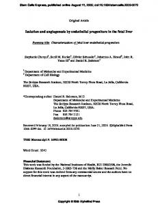
HOUR Fig. 1. Environmental hour-temperature relation on the 9 observation days; 3 coolest (O) and 3 warmest (O) days marked to show days used in Fig. 2. Glass mercury thermometer on surface of non-shaded ground (also at 7 cm deep, not

shown).

nests. (Method was checked by treating above on-the-hour counts for all replicate nests of a species as group for fitting a Lowess curve: the resultant species curve for any given species was almost identical to a species curve derived directly from original counts.) The same method was used for surface temperature, with curve fitted to counts over the temperatures; 8 "on-the-temperature" response variables (9, 12, 16, 23, 29, 34, 37, 40C) were chosen to span the range of environmental temperature and to correspond to the 8 hour variables. Deep-temperature response variables were derived in a similar way: 10, 12, 14, 16, 19, 22, 25, 28 C.

1990]

McCluskey & Neal--Ant diversity

67

In view of the high correlation between environmental temperature and hour (Fig. 1), how could response variables to these factors be distinguished?

1) Only morning observations were used, to avoid complications due to darkness-versus-light and to reversal from rising to falling temperature. 2) Some days were much warmer than others, thus partly decoupiing temperature from hour. 3) On the other hand, this makes it hard to interpret hour response variablesmthey were against a different temperature background every day. But in one case some uniformity was provided by combining counts for all the replicates of a species to give enough information to analyze the 3 warmest days separately from the 3 coolest days (Fig. 2). 4) Another approach was discriminant analysis. It considers responses (here, to temperature-hour environment) as a whole, using dependent (and often correlated) variables in concert. On the basis of known group membership it weights the variables so as to discriminate optimally among the groups (here, species) (Cooley & Lohnes 1971). Thus it could be used to test the variables for their part in diversity. Because conclusions are little better than the underlying replication (see Hurlbert 1984 for field studies), the types of"replicates" are listed. Though more than sometimes seen in field work, they were sufficient only for the exploratory analysis intended (see Williams & Titus 1988 for multivariate studies): Nests within species (Fig. 3). Species within profile analysis (Fig. 2). Coolest versus warmest days (Fig. 2). Profile comparison (Fig. 2) versus discriminant analysis (Fig. 3). Subgroups of variables in discriminant analysis (Fig. 3). RESULTS The most direct approach was to compare profiles shown as hour response with those shown as temperature response (Fig. 2). By either criterion the species patterns were distinctive. For example, the maxima for the bottom species were some 4 h later and 20 C

Psyche

68

[Vol. 97

1.2

0.6 SS

0.0

B 0,8

FZ

0.0

p

1.2

,,s 0.0 ’/ 0

III

"r,

K

-’ t"(.! s’

|

0.6 0.0

,,,.. . "’

;"

_.’

0.6

:/

0,0

F

,,

-"i

0.6

0.0 Hour 5.4 oC

3

7.5

9.6

13

23

11.7 33

COOLEST DAYS

5.4

7.5

9.6

12

20

28

11.7 36

13.8 44

WARMEST DAYS

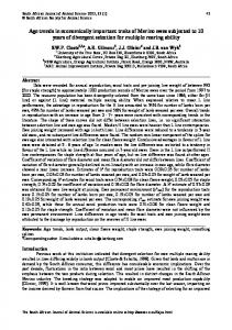
Fig. 2. Close correlation between responses (number of ants within 0.5 rn of nest entry) plotted in terms of hour (--) and of surface temperature (- -). To make such biological comparison unbiased, relation between hour and temperature scales on X axis was derived directly from environmental hour-temperature correlation. The 3 COOLEST and 3 WARMEST days (see Fig. l) form 2 independent checks of this comparison. Letter in corner of each panel: B Conomyrma bicolor, C Pogonomyrmex californicus, F and K Myrmecocystus flaviceps and kennedyi, H Pheidole barbara, P Messor pergandei (ants from 3 different subfamilies). Counts for all replicate nests of a species were treated as group and fitted by a Lowess curve. (Checking method by assigning half the replicates of each species to wrong species made hour-temperature correlation poor.)

1990]

McCluskey & NealmAnt diversity

69

higher than for the top ones (a big difference to an observer out in the sun!). But Fig. 2 shows how much alike the hour and temperature response patterns were for any one species. Even though ants were out earlier on the warmest than on the coolest days, there was the same detailed, species-specific correlation between hour and surface temperature response patterns. What could be done to separate temperature from hour variables? And central to the main topic here, how might enough species differences be found in just an 8-hour segment of the day to distinguish all 6 species? Discriminant analysis (Fig. 3) was used 1) to compare all species simultaneously, and hence 2) to test how completely they might be segregated by using many dependent variables. Either 8 hour, or 8 surface-temperature, or 8 deep-temperature response variables were tested. (It should be remembered that such a variable represents "response"--number outmof the ants at a particular hour or temperature.) In each case the species means differed (P