Mathematical Modeling Of Physical Processes In The Scroll ...

Purdue University

Purdue e-Pubs International Compressor Engineering Conference

School of Mechanical Engineering

2002

Mathematical Modeling Of Physical Processes In The Scroll Compressor Chamber S. Pietrowicz Shizuoka University

T. Yanagisawa Shizuoka University

M. Fukuta Shizuoka University

Z. Gnutek Wroclaw University of Technology

Follow this and additional works at: http://docs.lib.purdue.edu/icec Pietrowicz, S.; Yanagisawa, T.; Fukuta, M.; and Gnutek, Z., " Mathematical Modeling Of Physical Processes In The Scroll Compressor Chamber " (2002). International Compressor Engineering Conference. Paper 1589. http://docs.lib.purdue.edu/icec/1589

This document has been made available through Purdue e-Pubs, a service of the Purdue University Libraries. Please contact [email protected] for additional information. Complete proceedings may be acquired in print and on CD-ROM directly from the Ray W. Herrick Laboratories at https://engineering.purdue.edu/ Herrick/Events/orderlit.html

C20-6 MATHEMATICAL MODELING OF PHYSICAL PROCESSES IN THE SCROLL COMPRESSOR CHAMBER *Sławomir Pietrowicz 1, Visiting Researcher, Tadashi Yanagisawa 1, Professor, Mitsuhiro Fukuta 1, Associate Professor, Zbigniew Gnutek 2, Professor, 1

Shizuoka University, Department of Mechanical Engineering, 3-5-1, Johoku, Hamamatsu, Shizuoka, 432-8561, JAPAN Tel. /fax. +81- 53- 478 – 1058, E-mail: [email protected] *Author for Correspondence 2

Wrocław University of Technology, Institute of Heat Engineering and Fluid Mechanics, 27 Wybrzeże Wyspiańskiego Str. 50 – 370 Wrocław, POLAND Tel. +48 – 71- 302 – 3605, fax: + 48 – 71- 320 - 2076 E-mail: [email protected]

ABSTRACT Many mathematical models describing phenomena in the scroll compressors are based on the assumption that the state of working fluid is uniform in each scroll chamber and a change of the state proceeds according to the volume change as a function of time or the orbiting angle. Therefore, the models cannot predict the non-uniform distributions of velocity, temperature and pressure in the scroll chamber. In this paper, a numerical approach is adopted to predict two-dimensional distribution of the states of working fluid in the scroll chamber. The numerical analysis is based on equations of continuity, momentum and energy of fluid in the chamber. The space of the crescent-shaped scroll chamber is transformed into an orthogonal space system in which it is easy to imply the boundary conditions of the moving wall with temperature distribution. The calculation of the simultaneous differential equations is executed using commercial software MATHEMATICA and C++ and a thermophysical properties database REFPREX. The calculated results make clear, two-dimensional distributions of velocity and pressure, which gives good understanding about the physical processes in the scroll chamber.

NOMENCLATURE :enthalpy :Jacobian :turbulent energy :metrics :basic circle radius :radius of revolution :time :temperature :absolute velocity components :contravariant velocity components :Cartesian coordinate x&, y& :Cartesian component of the grid velocity

h J k q1, q2 rb re t T u, v U, V x, y

ε ρ µ µ eff η θ φ

:dissipation rate :density :absolute viscosity :diffusive coefficient :coordinate in the moving coordinate system :angular velocity of rotation :involute angle and one of the coordinates in the moving coordinate system

INTRODUCTION The scroll compressor is gaining the interest of manufacturers of air conditioners, cars etc. mainly due to its durability, low noise and relatively simple construction. Plenty of publications on this subject prove an interest of the researchers as well. Most of the papers are based on assumption that thermodynamic processes occurring inside the compressor are uniform and rely on mathematical formulas derived from the First Law of Thermodynamics. These formulae are in good correlation with experimental data but detailed analysis requires consideration of the non-uniform distributions of velocity and pressure. Due to the complexity of the processes, the only one way to get the results is solving the equations of continuity, momentum and energy using the numerical method. There are a few publications [4, 6, 8] about using numerical analyses in scroll geometry but they don’t show distribution of pressure and the method of implication of grid (especially orthogonal) adapted to the moving boundary conditions. Due to dynamics of the processes (high angular velocity) in this paper, the unsteady compressible viscous turbulent flow model [1,2] is used.

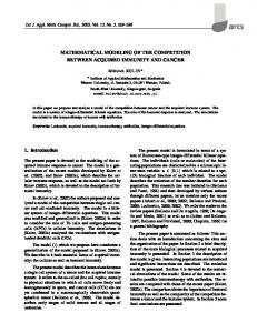
SPIRAL GEOMETRY Compressor geometry is described in many publications e.g. [7]. Figure 1 specifies all symbols describing scroll.

θ

θ

Figure 1. Outline of involute scroll wrap The scroll chamber can be characterized by parameterization equations:

x(φ ,η ,θ ) = rb (sin φ − φ cos φ ) + re (sin θ + η (cos φ − sin θ )) y (φ ,η ,θ ) = −rb (cos φ + φ sin φ ) + re (cosθ + η (sin φ − cos θ ))

(1a) (1b)

Families of curves are characterized by equations (1a), (1b) where every curve is parametrically described with respect to parameter φ and parameter η parameterizes family of curves. Parameter η changes in 0 ≤ η ≤ 1 interval, therefore for η = 1, the above equations describe the fixed wall and for η = 0, they describe the orbiting wall. The new coordinate φ, η is not orthogonal. The condition of curves orthogonality are expressed by dot product: xφ xη + yφ yη = 0 (2)

The new parameter – function of a (φ ) can be used instead of parameter φ, although for different curves (different η) another parameterization has to be used and function a (φ ,η ) depends on time θ – a (φ ,η ,θ ) . Thus this process can be described as follows: x new (φ ,η ,θ ) = x( a (φ ,η ,θ ),η ,θ ) (3a)

y new (φ ,η ,θ ) = y ( a (φ ,η ,θ ),η ,θ )

(3b)

Making use of the condition described by formulas (2), (3a) and (3b), relations for equation formula are derived:

a (φ ,η ,θ ) in differential

∂ a(φ , η, θ ) re cos(a (φ , η ,θ ) + θ ) = ∂η re φ − rb a (φ ,η , θ )

(4)

where initial condition a (φ ,0,θ ) = φ . This method was used to implicate an orthogonal grid within the scroll compressor chamber.

GOVERNING EQUATIONS IN A SCROLL CHAMBER Present study proposes a standard model of turbulent flow called the turbulent k-ε model, which was adapted to the new orthogonal coordinate φ− η. For: - continuity

∂ ( Jρ ) ∂ ( ρU ) ∂ ( ρV ) + + =0 ∂t ∂φ ∂η

(5)

- x-momentum

 ∂P ∂u  ∂u  ∂  µ eff ∂ ( Jρu ) ∂ ( ρUu ) ∂ ( ρVu ) ∂P  ∂  µ eff q1  + q2 + + = −  yη − yφ +  + SU (6)   ∂η  ∂φ  ∂η  J ∂t ∂φ ∂η ∂η  ∂φ  J  ∂φ

 µ eff SU = ∇ •   J

 ∂u ∂u  µ eff i +  yη − yφ ∂η  J  ∂φ

 ∂v ∂v    yη  j − yφ ∂η    ∂φ

(7)

- y-momentum

 ∂P ∂ ( Jρv) ∂ ( ρUv) ∂ ( ρVv) ∂v  ∂P  ∂  µ eff ∂v  ∂  µ eff q1  + q2 + + = − xφ − xη +  + SV (8)   ∂η  ∂η ∂φ  ∂φ  J ∂φ  ∂η  J ∂t ∂φ  ∂η  µ eff SV = ∇ •  −  J

 ∂v ∂v  µ eff i −  xη − xφ ∂η  J  ∂φ

 ∂v ∂v    j  xη − xφ ∂η    ∂φ

(9)

- enthalpy

∂ ( Jρh) ∂ ( ρUh) ∂ ( ρVh) ∂h  ∂  µ eff ∂h   dP  ∂  µ eff = J + + q1 q2 +  +   ∂η  ∂t ∂φ ∂η  dt  ∂φ  Jσ k ∂φ  ∂η  Jσ k

(10)

- turbulent energy

∂ ∂ ( Jρk ) ∂ ( ρUk ) ∂ ( ρVk ) = J (G + ρε ) + + + ∂φ ∂η ∂φ ∂t

 µ eff ∂k  ∂  µ eff ∂k  q2 q1  +   ∂η   Jσ k ∂φ  ∂η  Jσ k

(11)

- dissipation rate

∂ ( Jρε ) ∂ ( ρUε ) ∂ ( ρVε ) ε  ∂ + + = J  (C1G + C 2 ρε ) + ∂t ∂φ ∂η k  ∂φ

 µ eff ∂ε  ∂  µ eff ∂ε  q1  + q2    (12) ∂η   Jσ φ ∂φ  ∂η  Jσ φ

where J is the Jacobian of the coordinate transformation

J = xφ yη − xη yφ

(13)

velocities U and V are the contravariant velocity components. These velocities are defined as:

U = (u − x& ) yη − (v − y& ) xη

as:

(14)

V = (v − y& ) xφ − (u − x& ) yφ (15) In equations (14) and (15), the variables x& , y& are the Cartesian components of the grid velocity vector defined x& = ω re cos θ y& = ω re sin θ

(16)

q1 = xη2 + yη2

(18)

q 2 = xφ + yφ

(19)

(17)

The metrics q1, q2 are 2

2

The divergence of the coordinate transformation is defined as:

r  ∂F ∂F ∂F ∂F  ∇ ⋅ F =  yη 1 − yφ 1 + xφ 2 − xη 2  J ∂η ∂η ∂φ   ∂φ  2 G = µt  2  J

2 2 2  ∂u  ∂v   ∂v ∂u ∂u ∂v   1  ∂v ∂u      + 2  − xη  +  − xη − yφ + yη + xφ + xφ − yφ  yη ∂η   ∂φ ∂η ∂φ ∂η   J  ∂φ ∂η   ∂φ   

The diffusive coefficient is equal to:

µ eff = µ + µ t

(20)

(21)

(22)

Turbulent viscosity is defined as:

µt = ρ Cµ

k2

ε

(23)

According to publications [1,2], the various constants are: C1 = 1.44, C2=1.92, σk=1.0, σε = 1.3, Cµ = 0.09.

ASSUMPTIONS AND BOUNDARY CONDITIONS General assumptions: -

the working medium is the R22 gas; according to [3], temperature of the wall is distributed linearly with the involute angle φ and the temperatures of fixed and orbiting scrolls are equal to gas temperatures at the walls; the pressure gradient normal to the walls is set zero, ∂p ∂n = 0 ; the numerical calculations do not include tangential and radial leakages; gravity force is not taken into consideration;

Boundary conditions for velocity The geometrical relations of velocity on the moving wall are explained in Figure 2. The values of grid velocity are calculated using equations (16) and (17). The paper uses the following assumptions to simplify the velocity calculation procedure: - the absolute velocities on the fixed scroll are equal to zero; - non – slip condition is imposed at the end of the orbiting scroll (the contravariant velocities on the moving scrolls are equal to zero i.e. x& = u , y& = v ).

NUMERICAL CALCULATION PROCEDURE Generation of numerical grid Equation (4), describing orthogonal grid, is calculated using Runge-Kutta-Fehlberg method (Method RKF45). The process of evolving grid depending on angular velocity is presented in Figure 3.

Numerical procedures of calculations of continuity, momentum and energy For the compressor chamber space discretization 73x23 grid points were adopted. To carry out numerical calculation for equations (5)-(13), finite volume methodology was employed [1,2]. Staggered control volumes were used for the u and v equations. That is p, T and ρ values were stored at the center of main control volumes and u and v were stored at the faces in staggered control volumes. The SIMPLE algorithm described in [2] was employed in order to correct the pressure field.

RESULTS AND DISCUSION In this paper, numerical calculations were carried out for scroll compressor parameters specified in publication [7]. That are; basic circle radius rb= 3mm, wrap thickness b = 4.6 mm, radius of revolution re = 4.8 mm, crank shaft angular velocity ω = 366.5 rad/sec, wrap height hs=29.4 mm. The suction parameters are: ps = 584 kPa, ts=278.14 K. All calculations were executed in the commercial software, MATHEMATICA. To increase efficiency of calculation the main part of the program was written in C++ using standard procedures of MathLink. The same procedures were employed in order to calculate thermodynamic properties in REFPREX 6.0. Common points of orbiting and fixed scrolls are singularities at which Jacobian equals zero. Therefore the grid was diminished at these points. This end point truncation had negligible effect on the processes. Distribution of velocity, pressure and temperature for several crank positions is shown in figures 4, 5 and 6. From the calculations it was concluded that the highest absolute velocity within the scroll chamber occurs near the common points. The differences between the average and the highest velocities are considerable (Figures 4b, 5b, 6b). In addition, the highest-pressure gradient was observed near the common points. The differences between average and local pressure near the points amount to±250 Pa for θ =0 π to about ±450 Pa for points near the starting orbiting angle θ = −2.5 π Refer to Figures 4a, 5a, 6a. The highest temperature differences between orbiting, fixed and the gas occur at the initial compression stage (θ ≈ − 2.5 π). The heat is transferred from the walls to the working fluid. At the final stage, for θ ≈ 0 π, this phenomenon is changing its direction and the heat transfer goes from the gas to the walls. (Figures 4c, 5c, 6c)

CONCLUSIONS The study presents numerical solutions of thermodynamic processes occurring in a scroll chamber. In order to receive the complete description of phenomena an unsteady compressible viscous turbulent flow model in a moving coordinate system was proposed. Continuity, momentum, energy, dissipation rate and turbulent energy equations were discretized using finite volume methodology and were then adapted to staggered volumes. The simulations show large non-uniform pressure and velocity that prove significant variation of thermodynamic processes inside the scroll compressor. The results are theoretical and require providing an experimental database, although they represent the next step to a better understanding of these processes.

REFERENCES [1] Arakawa C. Computational Fluid Dynamics for Engineering, Tokyo, 1994. (in Japanese) [2] Fletcher C. A. J., Computational Techniques for Fluid Dynamics, Second Edition, Springer-Velag Berlin Heidelberg 1988, 1991.

[3] Jang K., Jeong S., “Temperature and heat flux measurement inside variable-speed scroll compressor,” 20th International Congress of Refrigeration, IIR/IIF, Sydney, 1999. [4] Morisita E. “Centrifugal fan operation of a co-rotating scroll compressor,” ASME, Vol. 222, Fluid Machinery, pp.167-172. [5] Shyy W, Francois M., Udaykumar H.S., “Computational moving boundary problems in engineering and biomechanics,” The 7th National Computational Fluid Dynamic Conference, Kenting, 2000. [6] Stosic N, Smith I. K. “CFD Studies of flow in screw and scroll compressors,” Proceedings of the 1996 International Compressor Engineering Conference at Purdue, pp.181-186. [7] Yanagisawa T., M. C. Cheng, M. Fukuta and T. Shimizu “Optimum operating pressure ratio for scroll compressors,” Proceedings of the1990 International Compressor Engineering Conference at Purdue, Vol. I, pp.425-433 (1990). [8] Zhu J., Ooi K.T, “Prediction of flow and heat transfer within a scroll compressor working chamber,” AES-Vol. 37., Proceeding of the AME Advance Energy System Division ASME 1997, pp.463-468.

Y

ν

.

x

.

y

−θ −θ

re X

ω moving scroll

ν

.

y

−θ

.

x

η

fixed scroll

φ

Figure 2. Velocities in the scroll system

Fixed

Orbiting 5 2

θ =− π

5 3

θ =− π

θ = 0π

5 6

θ =− π

Figure 3. The time-varying flow domain within the scroll compressor with the moving grid

a). Pressure

b). Velocity

c). Temperature

Figure 4. Pressure, velocity and temperature fields at orbiting angle θ = −

15 π 8

b). Velocity

a). Pressure

c). Temperature

5 8

Figure 5. Pressure, velocity and temperature fields at orbiting angle  θ = − π

a). Pressure

b). Velocity

c). Temperature

Figure 6. Pressure, velocity and temperature fields at orbiting angle

θ = 0π