Mathematical Modeling of Real-Time Scheduling for ... - SERSC

International Journal of Smart Home Vol. 9, No. 7 (2015), pp. 271-284 http://dx.doi.org/10.14257/ijsh.2015.9.7.28

Mathematical Modeling of Real-Time Scheduling for Microgrid Considering Uncertainties of Renewable Energy Sources Van-Hai Bui1, Nah-Oak Song2, Ji-Hye Lee1 and Hak-Man Kim1,* 1

2

Incheon National University Korea Advanced Institute of Science and Technology [email protected] Abstract

This paper deals with the real-time scheduling of a microgrid considering uncertainties of renewable energy sources (RESs). A two-step mathematical model based on real-time scheduling and demand responses (DRs) is proposed. DR programs, time of use (TOU) and emergency demand response programs (EDRP), are used to minimize the operation cost of microgrid. The proposed real-time scheduling is based on spinning and load reserves to deal with uncertainties of RESs. In the first step, the day-ahead scheduling is run for 24 hours with forecasted RESs. The second step deals with the actual RESs and the microgrid operation is rescheduled in the real time. The effectiveness of DR programs on the electrical demand for each interval is also shown in this study. The mixed-integer linear programming (MILP) method using CPLEX optimization program is used to solve the proposed two-step mathematical model. Keywords: Microgrid operation, demand response, TOU, EDRP, mixed-integer linear programming (MILP), day-ahead scheduling, real-time scheduling

1. Introduction A microgrid is the electricity distribution system, which usually consists of local loads, distributed energy resources including renewable energy sources (RESs), energy storage systems (ESSs). The use of RESs such as wind and solar power can bring economic benefits as well as improve environmental quality. However, it is difficult to forecast the exact amounts of the wind or solar power generations. The microgrid operation will be affected due to the uncertainties of wind or solar power generators. Therefore, it is necessary to consider the uncertainties of RESs in the microgrid operation [1-3]. Generally, a microgrid can be operated in grid-connected or islanded modes [4-6]. Gridconnected mode is considered in this study. The uncertainties of wind or solar power generators can be solved by using the spinning and load reserves in microgrids. The difference between the forecasted and actual outputs of RESs is compensated by these reserves. The real-time scheduling is used not only to minimize the total operation cost but also to ensure the stability of a microgrid system [7, 8]. The mathematical model of the real-time scheduling was proposed such as a two-stage model for real-time scheduling in [1, 3, 9] or short-term scheduling in [2]. Demand response (DR) programs are widely applied with real-time scheduling for the microgrid operation. While real-time scheduling can handle the problems introduced by uncertainties of RESs, DR programs can be implemented to reduce power demand during peak-interval as giving customers incentives or time-varying rates [10]. DR programs decide the amounts of shedding or shifting loads based on the market price and customers’ incentives for each time period [9, 11]. DR programs are divided into two categories: price-based programs and incentive-based programs. Time of use (TOU) *

Corresponding Author

ISSN: 1975-4094 IJSH Copyright ⓒ 2015 SERSC

International Journal of Smart Home Vol. 9, No. 7 (2015)

program is one of the price-based programs, which present rates with different unit prices for usage during different period. Emergency demand response program (EDRP) is a type of incentive-based DR program, which provides incentive payment to customers for reducing their loads during reliability-triggered events, but curtailment is voluntary [12]. Two DR programs, TOU and EDRP programs are considered for the microgrid operation in this study. The two step mathematical model of real-time scheduling based on the DR programs is proposed to solve the problems introduced by uncertainties of wind or solar power generators. The proposed model of real-time scheduling determines day-ahead generation scheduling and minimize the total operation cost of the microgrid with electrical and heat loads. In the first step, the day-ahead scheduling with the forecasted output amounts of RESs is performed by microgrid central controller (MGCC). In the second step, the realtime scheduling is run with the actual output amounts of RESs. The impact of DR programs on electrical loads and optimal microgrid operation is also shown in this study. The mixed-integer linear programming (MILP) method is used to solve the proposed twostep mathematical model using CPLEX optimization program under the C++ environment. The paper is organized as follows. In Section 2, the two steps mathematical model of real-time scheduling are proposed based on two demand responses, TOU and EDRP. Case study is presented in Section 3. Finally, conclusions and future works are summarized in Section 4.

2. Real-Time Scheduling for Microgrid Operation A microgrid consists of RESs such as wind or solar power generations. In practical, it is difficult to forecast the exact amounts of the RESs. Therefore, the uncertainties of wind or solar power generators need to consider in the microgrid operation. In this study, the two step mathematical model of the real-time scheduling is proposed to deal with the uncertainties of RESs, as shown in Figure 1. Step 1 is the day-ahead scheduling that considers the forecasted output amounts of RESs. Besides, Step 2 deals with the actual output amounts of RESs, and the uncertainties of RESs are compensated by spinning and load reserves. The real-time scheduling is run in Step 2 based on the difference of the forecasted and actual outputs of RESs. Additionally, in order to improve the stability of the microgrid, DR programs, which consist of TOU and EDRP programs, are applied to Step 1 to reduce the power demand during peak-interval. In order to apply DR programs, three types of loads depending on the types of the loads are assumed in this study, which are: fixed load, shiftable load, and controllable load as follows [13, 14]:  Fixed load (or non-controllable load): a demand that must be supplied to avoid user’s dissatisfaction.  Shiftable load: the load profile for these devices can be shifted from one period to another period for reducing demand load at peak hours.  Controllable load: loads cannot move to an interval from another and they must be on or off.

272

Copyright ⓒ 2015 SERSC

International Journal of Smart Home Vol. 9, No. 7 (2015)

Generator characteristic Forecasted output of RESs

Input data

Step 1: Day-ahead scheduling

Load Market price Input data

Actual output of RESs

Step 2: Rescheduling

Figure 1. Operation Process for Real-Time Scheduling 2.1. Nomenclature Before presenting the mathematical model of the microgrid operation, mathematical notations for the model are defined as follows: t = the identifier of operation interval T = the number of operation intervals i = the identifier of diesel I = the number of the diesel j= the identifier of CHP J = the number of the CHP k = the identifier of HOB K = the number of the HOB L c h a rg e

= losses for charging

L d is = losses for discharging

 j = the ratio of the heat and electric power of the j

= on or off mode of the i

u i (t )

C C

C

D ie se l i CH Pj

D ie s e l i

= the production cost of the k ( t ) = startup cost of the i

= startup cost of the i

C o n tr o l

In c s h e d

PR

S e ll

interval

diesel [won/kWh]

th

D ie s e l i

Buy

th

th

CHP

= the production cost of the j CHP [won/kWh]

C s ta r t

PR

diesel at t

= the production cost of the i

H O Bk

SU

th

th

(t )

th

th

th

HOB [won/kWh]

diesel at t

th

interval [won]

diesel [won]

= the incentive for load reduction at t

th

( t ) = the buying price from the power grid at t (t )

= the selling price to the power grid at t

Copyright ⓒ 2015 SERSC

th

interval [won/kWh] th

interval [won/kWh]

interval [won/kWh]

273

International Journal of Smart Home Vol. 9, No. 7 (2015)

th

th

p e n ( t fr o m , t to ) = penalty of shifting power from t fr o m interval to t to

interval

[won/kWh] Load

Pa d j

P

F ix

(t )

= the total amount of adjusted power load at t

th

interval [kWh]

( t ) = the amount of power consumed by the fixed load at t

S h ift

th

interval [kWh]

( t ) = the amount of power consumed by the shiftable load at t

Pin i

th

interval

[kWh] S h ift

Pa d j ( t )

= the amount of adjusted power consumed by the shiftable load at t interval after the load shifting [kWh]

P ( t fr o m , t to ) C o n tr o l

Pin i

th

th th = the amount of power shifted from t fr o m interval to t to interval [kWh]

( t ) = the amount of power consumed by the controllable load at t

th

interval [kWh] C o n tr o l

Pa d j

C o n tr o l

Ps h e d

P

RESs

(t )

= the amount of adjusted power consumed by the controllable load at th t interval after the load shedding [kWh]

(t )

= the amount of load shedding at t

th

interval [kWh]

( t ) = the output produced from renewable energy resources (RESs) at t

th

interval [kWh] P

P

H H

H H P

D ie s e l i

C H Pj

( t ) = the output produced from the i

th

diesel at t

( t ) = the electrical output produced from the j

C H Pj

( t ) = the heat output produced from the j

H O Bk

th

th

th

interval [kWh]

CHP at t

CHP at t

( t ) = the output produced from the i

th

HOB at t

Load

( t ) = the amount of heat demand at t

th

interval [kWh]

W a s te

( t ) = the amount of heat waste at t

Buy

th

th

th

th

interval [kWh]

interval [kWh]

interval [kWh]

interval [kWh]

( t ) = the amount of power purchased from the power grid at t

th

interval

[kWh] P

S e ll

(t )

= the amount of power sold to the power grid at t th

BESS

= the amount of power charged at t

BESS

( t ) = the amount of power discharged at t

Pc h a r g e ( t )

Pd is

BESS

Pm a x Pin i

BESS

interval [kWh]

interval [kWh] th

interval [kWh]

= maximum power capacity of the BESS [kWh]

BESS

PS o C

th

= initial power capacity of the BESS [kWh] ( t ) = state of charge (SoC) of BESS at t

th

interval [kWh]

IF

Pm a x ( t ) = maximum total amount of power shifting from another interval to

interval t [kWh] OF

Pm a x ( t ) = maximum total amount of power shifting from interval t to another

interval [kWh] D ie s e l i

Pm in

274

= minimum production capacity of the i

th

diesel [kWh]

Copyright ⓒ 2015 SERSC

International Journal of Smart Home Vol. 9, No. 7 (2015)

D ie s e l i

= maximum production capacity of the i

Pm a x

C H Pj

Pm in

= minimum production capacity of the j

th

C H Pj

Pm a x = maximum production capacity of the j

th

HOB [kWh]

H O Bk

= maximum production capacity of the k

P

RESs

th

HOB [kWh]

(t) = the difference of the RESs between forecasted and actual output at

t D ie s e l i

P

CHP [kWh] CHP [kWh]

= minimum production capacity of the k

Pm a x

diesel [kWh]

th

H O Bk

Pm in

th

th

interval [kWh] th

(t) = the difference of the i

diesel after rescheduling at t

th

interval

CHP after rescheduling at t

th

interval

[kWh] P

C H Pj

(t) = the difference of the

j

th

[kWh] P

Buy

(t) = the difference of buying after rescheduling at t

th

interval [kWh]

P

S e ll

(t) = the difference of selling after rescheduling at t

th

interval [kWh]

 Pd is

BESS

(t) = the difference of BESS’s discharging after rescheduling at t

th

interval [kWh]  Pc h a rg e (t) BESS

 Pa d j

Load

(t)

= the difference of BESS’s charging after rescheduling at t [kWh]

th

interval

= the difference of adjustable load after rescheduling at t

th

interval

[kWh] 2.2. Mathematical Model of Real-Time Scheduling The operation processes of MGCC consist of two steps, where the day-ahead scheduling and the real-time scheduling are dealt with. The day-ahead scheduling, which considers the forecasted output amounts of RESs, is run in Step 1. The real-time scheduling is run in Step 2 with the actual output amounts of RESs. 2.2.1. Step 1: day-ahead Scheduling Step 1 is the day-ahead scheduling of the microgrid with the forecasted output amounts of RESs. The spinning and load reserves are calculated based on the difference of forecasted and actual outputs of RESs. DR programs (TOU and EDRP programs) are applied in this step, which decide the amounts of loads shifting and shedding for reducing total cost objective function. The cost function of the microgrid in Step 1 is the total expenses occurred by the electric and heat energies for the microgrid as follows: M in C 

T

I

t 1

i 1

  C

D ie s e l i

P

D ie s e l i

D ie s e l i

( t )  C s ta r t

T  J C H Pj C H Pj   C P (t )  t 1  j 1

 SU

D ie s e l i

K



C

H O Bk

P

H O Bk

k 1

(t )



 (t )  

T

 [PR

Buy

(t )  P

Buy

(t )  P R

S e ll

(t )  P

S e ll

( t )]

(1)

t 1

Copyright ⓒ 2015 SERSC

275

International Journal of Smart Home Vol. 9, No. 7 (2015)

tb

T

  In c s h e d

( t )  Ps h e d

C o n tr o l

T

 

(t ) 

C o n tr o l

ta

[ p e n ( t fr o m , t to )  P ( t fr o m , t to )]

t fr o m  1 t to  1

T

I

  [ C re s e r v e (t)  Pre s e r v e (t)  Load

Load



t 1

D ie s e l

D ie s e l

C re s e r v ei (t)  Pre s e r v e i (t) ]

i 1

Constraints: The limited power of the diesel generator, CHP, and HOB are expressed by (2)(5): D ie s e l i

.u i ( t )  P

Pm in P

D ie s e l i

D ie s e l i

D ie s e l

(t )

D ie s e l i

( t )  Pre s e r v ei ( t )  Pm a x C H Pj

 P

C H Pj

( t )  Pm a x

H O Bk

 P

H O Bk

( t )  Pm a x

Pm in

Pm in

(2) .u i ( t )

(3)

CHPj

(4)

H O Bk

(5)

The ratio of the heat and electric power of CHP as following: C H Pj

H

(t)   j  P

CH Pj

(6)

(t)

On–off mode binary constraint: 1 u i (t )   0

if P

D ie s e l i

 0

(7)

o th e r w is e

The startup cost of a diesel unit is calculated as in (8) and (9): D ie s e l i

SU

D ie s e l i

( t )  C s ta r t

D ie s e l i

SU

 [ u i ( t )  u i ( t  1)]

(8)

(t )  0

(9)

The balance between the power supply and the power demand in the microgrid is expressed as in (10). When the BESS is discharged, it can be considered as the power supply in the microgrid. On the other hand, the BESS can be considered as the load when it is charged. The heat balance in the microgrid is given in (11). I

P fo r e c a s t ( t )  RESs



J

P

D ie s e l i

(t ) 



i 1

C H Pj

(t )  P

Buy

(t )  P

S e ll

( t )  Pd is

BESS

( t )  Pc h a rg e ( t )  Pa d j BESS

j 1

where Pa d j (t)  P Load

P

F ix

(t)  Pa d j (t)  Pa d j S h ift

C o n tr o l

J



C H Pj

(t) 

j 1



H

(t )

(10 )

(t)

K

H

Load

H O Bk

(t)  H

Load

(11 )

(t)

k 1

The amounts of charging and discharging of BESS are shown in (12) and (13), respectively. Equations (14) and (15) show the SoC of BESS for each interval. It means that the BESS should be operated in the allowable range. SoC in the first interval ( PSBo EC S S ) is the initial value of the BESS ( PSBo EC S S ( t  1)  PinBiE S S ). 0  Pc h a r g e ( t )  (1  L c h a rg e )  Pm a x BESS

BESS

0  Pd is

BESS

BESS

PS o C

( t )  PS o C

BESS

( t )  PS o C

BESS

( t  1)  Pd is

BESS

BESS

( t  1)

(12)

( t  1)  (1  L d is )

(13)

( t ) / (1  L d is )  Pc h a r g e ( t )  (1  L c h a rg e )

0  PS o C

BESS

276

 PS o C

BESS

( t )  Pm a x

BESS

(14) (15)

Copyright ⓒ 2015 SERSC

International Journal of Smart Home Vol. 9, No. 7 (2015)

The shiftable load can be shifted from peak intervals to off-peak intervals. It depends on the trading prices and generation costs. Equations (16)(17) express the constraints of th th the inflow power and the outflow power for shifting power from t fr o m interval to t to

interval. Shiftable power inflow constraint: T



P ( t fr o m , t )  Pm a x ( t ) IF

(16)

t fr o m  1 , t fr o m  t

Shiftable power outflow constraint: T



P ( t , t to )  Pm a x ( t )  Pin i OF

S h ift

(t )

(17)

t to  1 , t to  t

th th When the shiftable load is transferred from t fr o m to t to interval, the penalty is given as

follows:   p e n ( t fr o m , t to )    0

th

if c u s to m e r d o n ' t p e r m it s h ifta b le lo a d to t to

Equation (19) shows the amount of adjusted power after shifting load to t interval. T S h ift

Pa d j

(18)

o th e r w is e

( t )  Pin i

S h ift

T



(t )  t

fr o m



P ( t fr o m , t ) 

 1 , t fr o m  t

th

(19)

P ( t , t to )

t to  1 , t to  t

The amounts of power reduction and reserve for peak interval are shown in (20) and (21): ( t )  Pin i

C o n tr o l

C o n tr o l

Ps h e d

( t )  Pa d j

C o n tr o l

Pre s e rv e ( t )  Pa d j Load

C o n tr o l

The spinning and load reserves required for t

(20)

(t )

(21)

(t ) th

interval is given as follows:

I

Pre s e r v e (t)  Load



D ie s e l

Pre s e r v ei (t)  Pre s e r v e (t) m in

(22)

i 1

2.2.2. Step 2: Real-time scheduling In Step 2, the actual output amounts of RESs are measured, and the real-time scheduling is run based on the actual output amounts of RESs. The uncertainties of RESs are compensated by the spinning and load reserves that are determined in Step 1. The cost function of the microgrid in Step 2 is shown as follows: T

M in C 

I

  C

D ie s e l i

P

D ie s e l i

D ie s e l i

( t )  C s ta r t

 SU

D ie s e l i

(t )



t  t ' i 1

T  J C H Pj C H Pj   C P (t )  t  t '  j 1

K



C

H O Bk

P

H O Bk

k 1

 (t )  

(23)

T

 [PR

Buy

(t )  P

Buy

(t )  P R

S e ll

(t )  P

S e ll

( t )]

tt '

Copyright ⓒ 2015 SERSC

277

International Journal of Smart Home Vol. 9, No. 7 (2015)

tb





C o n tr o l

In c s h e d

( t )  Ps h e d

C o n tr o l

(t )

t  t ', t  a

The constraints for Step 2 are given in (24). The amounts of the spinning and load reserves are changed, which depend on the difference of the forecasted and actual outputs of RESs. The upper limited of load shedding and the output power of diesel generator are shown in (25) and (26), respectively. I

P

RESs

(t) 

J



P

D ie s e l i

i 1

(t) 



P

C H Pj

(t)   P

Buy

(t)   P

S e ll

(t)   Pd is

BESS

(t)   Pc h a rg e (t)   Pa d j BESS

Load

(t)

(24)

j 1

 Ps h e d P

C o n tr o l

( t )  Pre s e r v e ( t )

D ie s e l i

( t )  Pre s e r v ei ( t )

Load

(25)

D ie s e l

(26)

3. Case Study In order to show the validation of the proposed mathematical models for real-time scheduling in the microgrid, a case study has been conducted and its simulation results are presented in this section. 3.1. Scenario The microgrid in Figure 2 is used for case study of optimal microgrid operation; the microgrid consists of a photovoltaic power generator (PV), two diesel generators, two CHPs, a HOB. The BESS can be charged or discharged depending on the market price. Grid-connected operation mode of microgrid allows power trading with utility grid. The characteristics of distributed generators are presented in Table 1. While the forecasted output amounts of RESs are listed as in Table 2, the actual output amounts of RESs are in Table 3. Load data such as heat load and electrical load are shown in Table 4 and the market price is shown in Table 5. Table 1. Production Characteristics of Distributed Generators Item DG 1 DG 2 CHP 1 CHP 2 HOB

278

Cost (won/kWh) Variable Startup 100 75 35 35 150

200 175 150 150 200

Capacity (kW) Minimum Maximum 0 0 30 20 0

100 50 80 70 100

Copyright ⓒ 2015 SERSC

International Journal of Smart Home Vol. 9, No. 7 (2015)

Utility Grid DMS Microgrid

Electrical Load Shiftable Load

Fixed Load

Controllable Load

HOB

BESS

PV

Heat Load

EMS

Information flow Electrical energy Heat energy

Figure 2. Test Microgrid Table 2. Forecasted the Photovoltaic Power Generation Output Hour

1

2

3

4

5

6

7

8

9

10

11

12

Output (kWh)

0

0

0

0

55

75

130

150

170

200

220

250

Hour

13

14

15

16

17

18

19

20

21

22

23

24

Output (kWh)

230

200

140

100

80

0

0

0

0

0

0

0

Table 3. Real the Photovoltaic Power Generation Output Hour

1

2

3

4

5

6

7

8

9

10

11

12

Output (kWh)

0

0

0

0

55

100

145

170

180

200

210

215

Hour

13

14

15

16

17

18

19

20

21

22

23

24

Output (kWh)

210

200

175

100

60

0

0

0

0

0

0

0

Table 4. Load Data Hour

1

2

3

4

5

6

7

8

9

10

11

12

Electrical load (kWh)

400

400

395

397

420

455

460

475

490

510

550

600

Heat load (kWh)

100

100

120

123

125

120

130

135

135

140

140

135

Hour

13

14

15

16

17

18

19

20

21

22

23

24

Electrical load (kWh)

600

575

560

550

550

555

540

530

500

490

450

450

Heat load (kWh)

133

130

125

130

130

127

130

130

135

130

130

120

8 11 0

9 12 0

10 13 0

63

66

80

11 15 4 12 2

12 15 7 12 5

Table 5. Market Price Hour Buying price (won/kWh) Selling price (won/kWh)

Copyright ⓒ 2015 SERSC

1

2

3

4

5

30

33

41

54

67

15

15

22

34

45

6 7 4 5 1

7 7 8 5 5

279

International Journal of Smart Home Vol. 9, No. 7 (2015)

Hour

13

14

15

16

17

Buying price (won/kWh)

15 7 12 7

15 4 12 6

15 2 12 2

13 0

10 0

60

50

Selling price (won/kWh)

1 8 6 0 5 5

1 9 5 5 5 0

20

21

22

23

24

49

47

47

44

44

40

40

41

41

41

3.2. Day-ahead Scheduling In this case, the incentive for load shedding is assumed as 160 won/kWh. The microgrid can shift or shed their loads to the off-peak interval by MDCC to minimize their electricity payment. Figure 3 shows the day-ahead scheduling of microgrid with the forecasted output of RESs. Amounts of load shedding and load shifting are dispatched based on the market price by the DR programs. After implementing the DR programs, the load curve is changed as in Figure 3 drawn as a red solid line. The load in the peak interval is shifted to off-peak interval for reducing load demand. The outputs of the distributed generators are determined for power balance with the minimum total cost. BESS is charged during off-peak interval (interval 1, 2) due to the low buying price and is discharged during peak interval because of high buying price. PV CDG2 SELL

[kWh] 700

CHP1 Charging Modified load

CHP2 Discharging Original load

CDG1 BUY

600 500 400 300 200 100 0 -100 -200

1

2

3

4

5

6

7

8

9 10 11 12 13 14 15 16 17 18 19 20 21 22 23 24 Interval [hour]

Figure 3. Electric Part in Day-Ahead Scheduling In this step, the amounts of the reserves are calculated based on the difference between the forecasted and actual outputs of RESs. The minimum amounts of the reserves are determined for each interval based on historical data as shown in Figure 4. In this paper, diesel generators are used for spinning reserves as well as load reserves. The amounts of the reserves will be determined by the real-time scheduling for the stability of systems.

280

Copyright ⓒ 2015 SERSC

International Journal of Smart Home Vol. 9, No. 7 (2015)

CDG1_Reserve

Load_Reserve

Min_Reserve

[kWh] 60 50 40 30 20 10 0 1

2

3

4

5

6

7

8

9 10 11 12 13 14 15 16 17 18 19 20 21 22 23 24 Interval [hour]

Figure 4. Reserve Part in Day-Ahead Scheduling Figure 5 shows the amount of CHP and HOB outputs and heat load. It is always ensured that the balance between heat source and heat load for each period of time. Owing to the higher cost of HOB than the cost of CHP, HOB is used in case of the CHP cannot provide the heat load for peak interval. The amount of HOB output is usually small due to its high generation cost. The remaining heat is used to charge the heat energy storage system (HESS) which can be discharged for other intervals. However, in this case, the HESS is not useful because the amount of the remaining heat is small. CHP1

CHP2

HOB

Hwaste

LOAD

[kWh] 160 140 120 100 80 60 40 20 0 -20

1

2

3

4

5

6

7

8

9

10 11 12 13 14 15 16 17 18 19 20 21 22 23 24 Interval [hour]

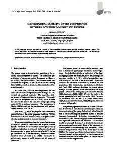
Figure 5. Heat Part in Day-Ahead Scheduling 3.3. Real-time Scheduling In this step, MGCC can measure the actual RESs output. The microgrid operation is rescheduled based on difference of the forecasted and actual outputs of RESs, as shown in Figure 6. When the amounts of actual outputs are greater than the forecasted outputs of RESs (at interval 6, 7, 8, 9, 15), the amounts of spinning and load reserves, external trading of electric energy with the power grid, the output power of generators, and charging or discharging of BESS are changed. In this case, the amounts of buying and the output power of generators are reduced to achieve the power balance. The spinning and

Copyright ⓒ 2015 SERSC

281

International Journal of Smart Home Vol. 9, No. 7 (2015)

loads reserves are used to compensate the difference of the forecasted and actual outputs of RESs. Additionally, these reserves can be used for the purpose of minimizing the operation cost based on the market price. For example, during peak interval, the selling price is greater than generator’s cost; therefore, the spinning reserves are sold to power grid to maximize the profits. Besides, when the amounts of the actual outputs of RESs are smaller than the forecasted outputs of RESs (at interval 11, 12, 13, 17), the amounts of buying power, load shedding, spinning reserves or the BESS power are changed to achieve the power balance as well as minimize the operation cost of the microgrid.

[kWh] 700

PV

CHP1

CHP2

CDG1

CDG2

Charging

Discharging

BUY

SELL

Modified load

Original load

600 500 400 300 200 100 0 -100

1

2

3

4

5

6

7

8

9 10 11 12 13 14 15 16 17 18 19 20 21 22 23 24 Interval [hour]

-200

Figure 6. Real-time Scheduling (Rescheduling)

4. Conclusions In this paper, a two-step mathematical model is proposed for real-time scheduling and demand response based on TOU and EDRP considering uncertainties. The differences between the forecasted and actual outputs of RESs are compensated by spinning and load reserves. Day-ahead scheduling is run in the first step based on the DR programs with the forecasted outputs of RESs and then the real-time scheduling is run in the second step with the actual outputs of RESs. The case study showed that the uncertainties of RESs are handled effectively by the two-step mathematical model and the economic operation of microgrid are achieved by the DR programs based on TOU and EDRP. As future works, the load forecasting model and the uncertainties of market price will be considered.

Acknowledgements This work was supported by the Power supply & Electricity Delivery Core Technology Program of the Korea Institute of Energy Technology Evaluation and Planning (KETEP), granted financial resource from the Ministry of Trade, Industry & Energy, Republic of Korea. (No. 20141020402350).

References [1]

[2]

282

S. Tanari, M. Reza Haghifam and A. Akhavein, “Optimization of the Microgrid Scheduling with Considering Contingencies in an Uncertainty Environment”, International Journal of Smart Electrical Engineering, Spring, vol. 2, no. 2, (2013), pp. 95-101. J. Soares, M. Silva, T. Sousa, Z. Vale and H. Morais, “Distributed energy resource short-term scheduling using Signaled Particle Swarm Optimization”, Energy, vol. 42, no. 1, (2012) June, pp. 466476.

Copyright ⓒ 2015 SERSC

International Journal of Smart Home Vol. 9, No. 7 (2015)

[3] [4]

[5] [6] [7] [8]

[9] [10] [11] [12] [13] [14]

P. Yi, I. Xinhua Dong and C. Zhou, “Real-Time Opportunistic Scheduling for Residential Demand Response”, Smart Grid, IEEE Transactions, vol. 4, no. 1, (2013) March, pp. 227-234. S-J. Choi, S-J. Park, D-J. Kang, S-J. Han and H-M. Kim, “A Microgrid Energy Management System for Inducing Optimal Demand Response”, Proceedings of IEEE International Conference on Smart Grid Communications, Brussels, Belgium, (2011) October 17-20, pp. 19-24. H.-M. Kim and T. Kinoshita, “A Multiagent System for Microgrid Operation in the Grid-interconnected Mode”, Journal of Electrical Engineering & Technology, vol. 5, no. 2, (2010) June, pp. 246-254. J-H. Lee and H-M. Kim, “LP-based Mathematical Model for Optimal Microgrid Operation Considering Heat Trade with District Heat System”, IJEIC, vol. 4, no. 4, (2013), pp. 13-21. Z. Zhao and L. Wu, “Impacts of High Penetration Wind Generation and Demand Response on LMPs in Day-Ahead Market”, Smart Grid, IEEE Transactions, vol. 5, no. 1, (2014) January, pp. 220-229. L. Lu, J. Tu, C.-K. Chau, M. Chen, Z. Xu and X. Lin, “Towards real-time energy generation scheduling in microgrids with performance guarantee”, Power and Energy Society General Meeting (PES), (2013) July 21-25, pp. 1-5. A. Zakariazadeh and S. Jadid, “Smart microgrid operational planning considering multiple demand response programs”, AIP Publishing, vol. 6, no. 1, (2014). J. O’Neill, Editor, “Demand Response Electricity Market Benefits and Energy Efficiency Coordination”, Published by Nova Publishers, Inc. New York, (2013). H. A. Aalami, M. Parsa Moghaddam and G. R. Yousefi, “Modeling and prioritizing demand response programs in power markets”, Electric Power Systems Research, vol. 80, no. 4, (2010) April, pp. 426-435. M. QamarRaza, M. UsmanHaider, S. Muhammad Ali, M. Zeeshan Rashid and F. Sharif, “Demand and Response in Smart Grids for Modern Power System”, SGRE, vol. 4, no. 2, (2013) May, pp. 133-136. A. Parisio and L. Glielmo, “A mixed integer linear formulation for microgrid economic scheduling”, Smart Grid Communications (SmartGridComm), (2011) October 17-20, pp. 505-510. P. Stluka, D. Godbole and T. Samad, “Energy management for buildings and microgrids”, Decision and Control and European Control Conference (CDC-ECC), (2011) December 12-15, pp. 5150-5157.

Authors Van-Hai Bui, he received B.S. degree in Electrical Engineering from Hanoi University of Science and Technology, Vietnam in 2013. Currently, he is a combined Master and Ph.D. student in the Department of Electrical Engineering, Incheon National University, Korea. His research interests include microgrid operation and energy management system (EMS).

Nah-Oak Song, she received her B.S. and M.S. degrees from Yonsei University, Korea, in 1989 and 1993, respectively, and the Ph.D. degree from the University of Michigan, Ann Arbor, USA in 1999. She worked for Samsung Electronics, Korea, from 1999 to 2001; the National Institute of Standards and Technology (NIST), USA, from 2001 to 2004; and the Electronics and Telecommunications Research Institute (ETRI), Korea, from 2004 to 2006. Currently, she is a research professor at Korea Advanced Institute of Science and Technology (KAIST), Korea. Her research interests include Energy Management System, Microgrids, V2G, and communication networks with emphasis on PLC, WLAN, and resource optimization.

Ji-Hye Lee, she received B.S degree and M.S degrees in Electrical Engineering from Incheon National University, Korea, in 2012 and 2014, respectively. Currently she is a Ph.D. course student in the Department of Electrical Engineering, Incheon National University, Korea. Her research interests include energy management system (EMS), optimal operation of microgrid and smart energy network.

Copyright ⓒ 2015 SERSC

283

International Journal of Smart Home Vol. 9, No. 7 (2015)

Hak-Man Kim, he received his first Ph.D. degree in Electrical Engineering from Sungkyunkwan University, Korea in 1998 and received his second Ph. D. degree in Information Sciences from Tohoku University, Japan, in 2011, respectively. He worked for Korea Electrotechnology Research Institute (KERI), Korea from Oct. 1996 to Feb. 2008. Currently, he is a professor in the Department of Electrical Engineering and also serves as the Vice Dean of College of Engineering, Incheon National University. His research interests include microgrids, LV/MV/HVDC systems.

284

Copyright ⓒ 2015 SERSC