Mathematical modeling of spreading cortical

American Institute of Physics Conf. Proc., Vol. 1028, pp 46-64 (2008).

Mathematical modeling of spreading cortical depression: spiral and reverberating waves Henry C. Tuckwell Max Planck Institute for Mathematics in the Sciences Inselstr. 22, Leipzig, D-04103 Germany Abstract. Mathematical models of spreading depression are considered in the form of reactiondiffusion systems in two space dimensions. The systems are solved numerically. In the two component model with potassium and calcium ion concentrations, we demonstrate, using updated parameter values, travelling solitary waves of increased potassium and decreased calcium. These have circular wavefronts emanating from a region of application of potassium chloride. The collision of two such waves does not, as in one space dimension, result in annihilation but the formation of a unified wave with a large wavefront. For the first time we show that the mathematical model reproduces the actual properties of spreading depression waves in cortical structures. With attention to geometry, timing and location of stimuli we have succeeded in finding reverberating waves matching experiment. By simulating the technique of anodal block, spiral waves have also been demonstrated which parallel those found experimentally. The six-component model, which contains additionally sodium, chloride, glutamate and GABA, is also investigated in 2 space dimensions, including an experimentally based exchange pump for sodium and potassium. Solutions are obtained without (amplitude 29 mM external K+ ) and with action potentials (amplitude 44 mM external K+ ) with speeds of propagation, allowing for tortuosity, of 1.4 mm/minute and 2.7 mm/minute, respectively. When action potentials are included a somewhat higher pump strength is required to ensure the return to resting state. Keywords: Spreading depression, brain dynamics, ion and transmitter movements, migraine PACS: 84.35.+i, 87.10.+e, 87.16.Ac

INTRODUCTION Spreading depression (SD) is a complex wave of transient depolarization of neurons and glia that propagates across cortical and subcortical gray matter at speeds of 2-5 mm/min. It arises mainly as a response to brain injury or pathology. By itself SD does not usually damage brain tissue, but during stroke and head trauma SD can arise repeatedly near the site of injury and may promote neuronal damage. One of the characteristics of SD is a large increase in extracellular potassium and a dramatic fall in extracellular calcium and other ions [1,2]. For reviews, see [3,4]. There has been much evidence for the idea that SD is a concomitant or cause of migraine [5-7]. A strong link exists between glutamate and migraine [8] and glutamate has been found to be important in the propagation of SD [9]. SD is associated with focal ischemia, traumatic brain injury [10,11], seizure activity [12] and spinal cord injury [13]. New effects and roles for SD have been discovered in the last several years. It has been demonstrated in human neocortical slices [14], has been found to suppress γ -activity in rabbit cortex [15] and it has been elicited in the brainstem [16], thought previously not to be capable of supporting SD. SD has also been recently shown to

release ATP into the extracellular compartment [17] and sustained elevated levels of potassium ion concentration have been found to lead to significant amounts of neuronal death [18]. Another finding, revealed by MRI, is that SD has components called primary and secondary events, the former having greater range and greater speed [19]. SD involves neuronal, including synaptic, and glial elements and there are a very large number of physiological and anatomical details which are relevant to its propagation, all of which are difficult to include in a mathematical model. These details include those of the dynamics of many neuronal and glial ion channels, pumps and other clearance mechanisms, blood supply, gap junctions as well as diffusion in the extracellular space. Just the aspects of presynaptic terminals and the dynamics of transmitter release are extremely complex as there are hundreds of different channel types in these specialized parts of the nervous system [20]. Glia and neurons are connected by gap junctions which are ubiquitous in brain circuits [21]. Some gap-junction blockers have been found to impede SD, resulting in reduced amplitude and duration [22]. The NMDA blocker MK801 was found to prevent SD in mouse neocortical slices but not an accompanying astrocytic calcium wave, though its speed was reduced [23]. Further, the specific gap junction blocker carbenoxolon did not prevent SD but also reduced the speed of the calcium wave. It is noteworthy that increased potassium reduces the efficacy of NMDA receptor antagonists to block SD [11]. There appears to be a reciprocal interaction between neurons and glia through neurotransmitter release, uptake and calcium fluxes [24, 25]. Astrocytes have been found to play a role in the modulation of synaptic inhibition [26] and glia have been suggested as playing an important role in SD [27]. However, the effects of gap junction blockers may be more than just blocking gap junctions, which clouds the role of gap junctions in SD. For example, some alcohols have been shown to affect both receptor-activated ion channels and voltage-gated ion channels [28]. These effects include inhibition of subtypes of NMDA-glutamate receptor ion channels and potentiation of certain subtypes of GABA-A receptor ion channels. Altered properties of these and other ion channels may contribute to the difficulty of eliciting SD in the presence of gap-junction blockers. Furthermore, alcohols may change the probabilities of opening of sodium channels [29, 30]. Mathematical models of SD have usually taken the form of reaction-diffusion systems - that is systems of parabolic partial differential equations involving spatial diffusion, with one or several equations for each neurochemical variable. Solutions of the equations are obtained by numerical methods, although some useful information about solution properties can be obtained analytically for the simpler models. Theoretical and experimental aspects of reaction-diffusion systems in the brain have been comprehensively reviewed by Nicholson [31]. Properties of reaction-diffusion systems in other areas such as the BelousovZhabotinsky reaction [32] may extend to neural phenomena including SD. Computational models of SD have sometimes adopted the cellular automata approach which is a useful first approximation [33,34]. Properties of SD, such as topographical constraints, have also been usefully investigated with mathematical models of general excitable systems, typified by the Fitzhugh-Nagumo equations [33, 35-37] and metabolic models have been related to migraine aura [38]. Shapiro’s [39] model included a great amount of physiological detail including gap-junctional mechanisms and volume changes.

Continuum neural models have mathematical properties of interest, such as travelling wave solutions [40] and pattern formation [41]. Theoretical models of SD include those which incorporate a single-cell approach [42,43], which is useful for delineating local effects, and electrodiffusion models [44]. In this article we consider some properties of reaction-diffusion models with 2 and 6 components in two space dimensions in order to investigate their properties and to demonstrate for the first time the experimental phenomena of spiral waves and reverberating waves for SD.

THE SIMPLIFIED TWO-COMPONENT MODEL IN TWO SPACE DIMENSIONS Diffusion through brain extracellular space proceeds quite readily even for larger molecules [48,49] so there is doubtless a substantial contribution to the propagation of SD by diffusion. This is supported by the fact that models which allow for diffusion and tortuosity give the correct speed for SD. Significant changes in extracellular space occur during SD [50,51] but these changes are neglected here because we concentrate mainly on low-amplitude waves and moderate changes in external K + have little such effect [52,53]. In the simplified model in two space dimensions, with extracellular potassium and calcium ion concentrations, denoted by K o (x, y,t) and Cao (x, y,t), playing key roles, the model equations are as follows, slightly modified from [46],

∂ Ko = DK ∇2 K 0 + f (K o ,Cao ) ∂t ∂ Cao = DCa ∇2Cao + g(K o ,Cao ) ∂t where ∇2 = ∂∂x2 + ∂∂y2 , DK and DCa are diffusion coefficients and f and g are the reaction terms to be described below. To reduce the number of differential equations with little loss of accuracy the corresponding internal concentrations are given by 2

2

K i (x, y,t) = K i,R − Cai (x, y,t) = Cai,R −

¤ α£ o K (x, y,t) − K o,R β ¤ α£ o Ca (x, y,t) −Cao,R γ

where the superscript R denotes resting level and where α /β and α /γ are ratios of the volume of extracellular space to those of the appropriate intracellular compartments. For potassium, contributions to f come from flux into postsynaptic compartments and a pump which acts to restore resting ionic concentrations. We may put f = fsource − f pump where fsource = k1 (VK −V )(V −VCa )gCa (V ) and

£ © ª¤ f pump = k2 1 − exp − k3 (K o (x, y,t) − K o,R ) .

FIGURE 1. Showing the extracellular potassium ion concentration at t=2.5 and t=5.0 for the twocomponent model with standard parameters.

Here VK and VCa are the Nernst potentials for potassium and calcium VK =

RT ln(K o /K i ) F

RT ln(Cao /Cai ) 2F and V is the equilibrium membrane potential · o ¸ RT K + pNa Nao + pCl Cl i V= ln F K i + pNa Nai + pCl Cl o VCa =

where Nai,o , Cl i,o are the appropriate internal and external concentrations of sodium and chloride ions and pNa , pCl are the corresponding relative permeabilities. gCa (V ) is the calcium conductance of presynaptic membrane, given by gCa (V ) = [1 + tanh[k7 (V +VT )] − k8 ]H(V −Vc ) where Vc is a cut off voltage and putting k8 = 1 + tanh(k7 (Vc + V T )) ensures that the conductance rises smoothly from zero. H(x − xo ) is a unit step function at xo . Similarly we put g = g pump − gsink where gsink = k4 (VCa −V )gCa (V )

FIGURE 2. Showing the extracellular calcium ion concentration (looking from below) at t=2.5 and t=5.0 for the two-component model with standard parameters.

£ © ª¤ g pump = k5 1 − exp − k6 (Cao −Cao,R ) . The value of RT F is chosen appropriately for 37 degrees Celsius. All concentrations are in mM. What we will call the standard parameter set consists of the following: k1 = 3.3, k2 = 208, k3 = 10, k4 = 0.3, k5 = 2.38, k6 = 40, k7 = 0.11, K i,R = 140, K o,R = 3, Cai,R = 0.0001, Cao,R = 1, VT = 45 mV, Vc = −70 mV, α /β = 0.53, α /γ = 0.207. The accepted value for the fraction of the brain which is extracellular space is 0.2 [49] so the values of α /β and α /γ differ considerably from those used previously, being based on [54]. Note that the actual intracellular volumes are not necessarily those available for occupation by ions and molecules because of various intracellular organelles such as mitochondria, filaments and other elements. The model was tested with large ranges for these parameters. Since here sodium and chloride movements are ignored, in contrast with the 6-component model, the quantities

γ = pNa Nao + pCl Cl i δ = pNa Nai + pCl Cl o are held fixed at 9 mM and 40 mM, respectively. The quantity RT /F is set at 60.09. Numerical integration is performed on x ∈ [0, 2.5], y ∈ [0, 2, 5] with an explicit method and the results were checked against those for an implicit method. For the numerical integration ∆x = ∆y = 2.5/300 and ∆t = .005. (Distances are scaled so that the diffusion coefficients are 0.0025 and 0.00125 for potassium and calcium.) With the standard set of

FIGURE 3. Showing the extracellular potassium ion concentration during a collision in the two component model with standard parameter set. The times indicated are tk = 200, 400, 600 & 900.

o = 17.14 mM and Cao = 0.04 parameters, a stable solitary wave with amplitude Kmax min mM formed from supra-threshold local elevations of external potassium

· o

K (x, y, 0) = K

o,R

+ 20 exp −

½µ

x − 1.25 0.05

¶2

µ

y − 1.25 + 0.05

¶2 ¾¸ ,

with Cao (x, y, 0) = Cao,R . Throughout the paper, a unit of distance corresponds to about 5.2 mm and a unit of time is about 26 seconds [47]. The discrete time points are denoted by tk , k = 0, 1, ..., T /∆t. Figures 1 and 2 show potassium and calcium waves for standard parameters when action potentials are ignored.

Collision In Figure 3 is shown the result for a collision between two SD waves, one starting at (x, y) = (1.05, 1.05) and the other at (x, y) = (1.45, 1.45). It can be seen that after colliding the waves merge to form a wave of a large wavefront, unlike the case in 1 spatial dimension where colliding waves annihilate.

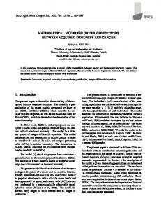
Reverberating SD waves One very interesting aspect of waves of spreading depression was the demonstration of reverberating waves; that is, waves which keep circling an obstacle for a very long time. In the experiments [55] in rat cortex, spreading depresssion waves could circulate for several cycles, with more cycles when lesions were made in some regions than others. On occasion, up to 27 cycles were observed. The principal method of instigation of reverberating SD was with the topographical set up of Figure 4. As depicted in A, a lesion or obstacle Q of large enough dimension is made in the cortex. A suitable stimulus, such as a local increase of potassium chloride concentration sufficient to elicit a wave, is applied at S1. After a certain time interval, the wavefront has split into two components W1 and W2 on either side of Q. At this point a second stimulus S2 is applied so that its emitted waves move on one side into the refractory zone of W1 and on the other side into the recovered zone in the wake of W1. If the timing and location of the second stimulus are appropriate, then as shown in B the first waves have passed the obstacle as wavefront W3 and meanwhile the surviving part of the secondary wave is at U1. In C, the first wave has reached the boundary as W4 where it will die and the secondary wave has advanced to U2. Hereafter, as in D, the secondary wave is able to circulate unimpeded around the obstacle. In experimental reverberating SD, the wave motion starts to slow after several cycles and eventually disappears due to exhaustion of local metabolic resources after successive recoveries from SD. This latter aspect is not addressed with the present model but it could possibly be incorporated in a model such as that of [56, 57] where metabolic variables were included in a model of stroke which embraced SD. The computational details for a reverberating wave are as follows. The model equations were as in the beginning of Section 2 with what we have called the standard parameter set. The rectangle x ∈ [0, 0.8] and y ∈ [0, 0.9] is used with an obstacle centered at x = 0.4, y = 0.45 with radius 0.2. The increments in ∆x, ∆y and ∆t are 0.8/60, 0.9/70 and 0.01, respectively. At t = 0 increased potassium (chloride) was applied as £ ¡ ¢¤ K o (x, y, 0) = K o,R + 20 exp − ((x − 0.4)/0.05)2 + ((y − 0.725)/(0.05))2 , with Cao (x, y, 0) = Cao,R . The resulting wave pattern was observed and it was noted when one branch of the primary wave was at W1 as indicated in Figure 4A. There was not much freedom in the timing and location of the second stimulus S2. Several placements led to a non-clean secondary wave which left behind a small patch of increased potassium that developed into a complex wave pattern. Thus after several attempts the following second stimulus was found to lead to a clean SD wave emanating from S2 in the back direction K o (x, y, 281∆t) = K o (x, y, 280∆t) £ ¡ ¢¤ +10 exp − ((x − 0.7)/0.06)2 + ((y − 0.44)/(0.06))2 , and Cao (x, y, 281∆t) = Cao (x, y, 280∆t). The results are shown in plan view in Figures 5 and 6 and parallel those in experimentally produced reverberating waves in retinal SD. At the 20-th time point (tk = 20), the initial Gaussian distribution has spread a

FIGURE 4. The topographical setup for obtaining reverberating waves of spreading depression. In A is shown a brain region containing a lesion or obstacle Q which blocks the passage of SD. S1 is the first stimulus which gives rise to waves W1 and W2 which pass around the obstacle. At a suitable time and location, a second stimulus S2 is applied in the back of the first wave W1. As shown in B, this wave can only move to the right which it does into a non-refractory zone. Meanwhile the first waves advance firstly to W3 and then as seen in C to the boundary of the region where they die, leaving the sole SD wave to circulate unimpeded as in D.

small amount and, by tk = 150, two SD wavefronts are observed travelling in opposite directions away from the source. At tk = 280 the wavefronts are at about the narrowest part of the region between obstacle and boundary and this is when the second stimulus is applied at tk = 281 - see the bottom right part of Figure 5. At tk = 500 (see Figure 6), the initial two wave branches waves are merged and about to pass into the left-hand boundary at y = 0 where they are absorbed whereas the secondary wave is seen travelling at top right on its first circuit of the obstacle. At tk = 700 the sole secondary wave can be seen travelling down past the right side of the obstacle and it continues indefinitely, in the absence of metabolic constraints, in a clockwise motion about the obstacle.

Spiral SD waves Spiral waves are frequently found in reaction-diffusion systems involving excitable and recovering elements [41, 35, 58] and there have been many theoretical attempts to understand them [59-61]. Experimentally they have been observed for SD in chicken retina [62, 63]. However they have never been obtained in bona fide models of spreading depression so we decided to investigate their possible occurrence in the improved

FIGURE 5. Showing the first phases of the development of a reverberating SD wave as seen in experiments on rat cortex. For parameter values, see text.

FIGURE 6.

Showing the established reverberating SD wave.

FIGURE 7.

Showing the set up for development of a spiral wave of SD. For full explanation, see text.

two-component model outlined above. Time did not allow their investigation in more complex models. In one set of spreading depression experiments carried out on chicken retina, the method of anodal block was used to extinguish a part of an SD wavefront [62]. The end of remaining part of the wave curled around behind the almost plane-wave front to give a spiral. This could be done by dissolving one end of a wave or a middle segment. In the latter case two spirals lurched towards each other. To study this phenomenon it is necessary to effect the mathematical equivalent of an anodal block. There are doubtless several ways to do this, but the following was adopted. A wave is started at point P in Figure 7 in the lower left quadrant. A block of all entry of an SD wave into the lower right (shaded) quadrant is effected by holding the ionic concentrations at their resting levels until the time when the wavefront from the source at P is just at the upper edge RS of the lower left quadrant. At this instant the clamp on the lower right quadrant is removed, leaving a wavefront along RS with a completely unrefractory region to its right and a refractory region immediately behind it. At the time of the removal of the clamp, the set up is equivalent to having extinguished the right branch of a travelling wavefront. The results of the computations are shown in Figure 8. The region considered is x ∈ [0, 2], y ∈ [0, 2] with 151 space points in both x and y directions. The time step is 0.01. The lower right quadrant was held at the resting level until tk = 400 and a wave started with the initial distribution £ ¡ ¢¤ K o (x, y, 0) = K o,R + 20 exp − ((x − 0.3)/0.05)2 + ((y − 0.5)/(0.05))2 concentrated in the center of the lower part of the bottom left quadrant. The wave front becomes almost a plane wave front at tk = 450 (t = 4.5) occupying approximately the

tk=450

tk=900

FIGURE 8. Showing the development of a spiral wave as seen in experiments on retinal spreading depression. The graphics has distorted the wavefronts which are actually circular. For remaining parameter values, see text.

upper boundary of the lower left quadrant as seen in the Figure. At tk = 600 the right hand end of the wave has begun to curl around behind the plane wave and this spiralling continues for several turns until the simulation is terminated at tk = 900. Note that these spirals are actually circular but the graphic limitations have made them appear rather squarish. The spiralling is exactly analogous to that found in experiments with the anodal block technique.

THE 6-COMPONENT MODEL WITH K + , Ca++ , Na+ , Cl − AND EXCITATORY AND INHIBITORY TRANSMITTERS The above two-component model is useful for studying certain phenomena associated with spreading depression. However, a more extensive model [47] considers the 4 ions K + , Ca++ , Na+ , Cl − and an excitatory transmitter, denoted by TE , which is expected to be mainly glutamate, and an inhibitory transmitter, denoted by TI , mostly GABA. Letting the vector of external ion and transmitter concentrations be u(x, y,t) with u1 , ..., u6 , as those of K + , Ca++ , Na+ , Cl − , TE and TI , respectively, then quite generally

∂u = ∇2 u + F(u) ∂t with an initital condition u(x, y, 0) = u0 (x, y),

and suitable conditions at the boundary of the region under consideration. SD is actually a phenomenon in 3 space dimensions, but we consider only two for economy of computation. We consider two intracellular compartments, one pertaining to synapses and the other to nonsynaptic processes which may include contributions from glia. These are assigned possibly different ratios of extracellular to intracellular volumes, denoted by α1 and α2 , respectively. The internal ion concentrations, denoted by uint i , i = 1, 2, 3, 4, are assumed to be given by the local conservation equations, which for potassium, sodium and chloride are, with R denoting a resting equilibrium value, int,R uint + α1 [uRi − ui (x, y,t)], i = 1, 3, 4, i (x, y,t) = ui

for potassium, sodium and chloride whereas for calcium int,R uint + α2 [uR2 − u2 (x, y,t)]. 2 (x, y,t) = u2

It is more transparent to use K o,i , Cao.i , Nao,i , Cl o,i , TEo,i and TIo,i for the ion and transmitter concentrations and it is expeditious to omit the space-time coordinates (x, y,t). The membrane potential is assumed given by the Goldman formula · o ¸ K + pNa Nao + pCl Cl i RT VM = ln F K i + pNa Nai + pCl Cl o and the Nernst potentials are as given in Section 2 for K and Ca and by similar formulas for Na and Cl. The very complex dynamics of calcium at presynaptic terminals have been the subject of many experimental and theoretical studies mainly with a view to quantitatively understanding transmitter release [64-66]. Other works have concentrated on calcium dynamics in neurons during action potentials [67]. We include a major component of calcium fluxes, that associated with the activation of synapses because of its relevance to transmitter release. Although flows through other membranes are doubtless significant they are for the most part neglected in the present model. Their inclusion is no more difficult and their quantitative aspects just as uncertain but to maintain a degree of simplicity they are omitted. The source and sink terms are slightly modified from those given in [46]. For potassium, ¸ · k3 TIo TEo + − PK,Na + fK,p + k5 , fK = k1 (VM −VK ) o TE + k2 TIo + k4 where PK,Na is the pump term and fK,p is a passive flux term given by fK,p = k6 (VM −VM,R )(VM −VK )H(VM −VM,R ) where VM,R is resting membrane potential. The constant k5 ensures that fK = 0 at resting levels and it is assumed that the transmitter induced conductance changes are zero unless TEo , TIo are positive. Although ion pumps have a complicated dependence on concentrations of several ion species [68,69], we have adopted a model with an explicit

and relatively simple form for the sodium-potassium exchange pump [70], ¶ µ ¶ µ k19 −2 k18 −3 1+ o , PK,Na = k17 1 + i Na K where it is assumed that Nai > 0 and K o > 0. For calcium, fCa = k7 (VM −VCa )gCa + PCa − k8 where the calcium conductance is gCa = (1 + tanh[k31 (VM +VM∗ )] − k32 )H(VM −VMT ), VMT being a cut-off potential with k32 = 1 + tanh[k31 (VMT +VM∗ )] to ensure gCa rises smoothly up from zero as VM increases through VMT . The calcium pump is simply k20Cai H(Cai ) PCa = . Cai + k21 The sodium and chloride terms contain transmitter-induced conductance changes and pumps ¸ · TEo k10 TIo + − k22 PK,Na − k11 fNa = k9 (VM −VNa ) o TE + k2 TIo + k4 · ¸ k13 TEo TIo fCl = k12 (VM −VCl ) o + + PCl − k14 TE + k2 TIo + k4 where

k25Cl i H(Cl i ) . Cl i + k26 Glutamate NMDA receptors have been strongly implicated in SD as known blockers of them prevent SD [71,72]. Rates of transmitter release are assumed proportional to calcium flux so fTE = k15 (VM −VCa )gCa − PE PCl =

fTI = k16 (VM −VCa )gCa − PI , where PE =

k27 TEo H(TEo ) TEo + k28

k29 TIo H(TIo ) PI = . TIo + k30 Glutamate may also be released from glia during SD [73,74], but this contribution is not explicitly taken into account here. The pump terms for glutamate and GABA represents the clearance of these transmitters, for example into glial cells [75].

Results with the standard parameter set The above system of six reaction-diffusion equations was integrated using an explicit method. In particular, the first results are obtained with the following set of constants called the standard set.

Ratios of extracellular to intracellular volumes α1 = 0.25, α2 = 2.0. Diffusion coefficients in units of 10−5 cm2 sec−1 DK = 2.5, DCa = 1.0, DNa = 1.7, DCl = 2.5, DTE = DTI = 1.3. Resting concentrations in mM K o,R = 3, K i,R = 140,Cao,R = 1,Cai,R = 0.0001, Nao,R = 120 Nai,R = 15,Cl o,R = 136.25,Cl i,R = 6. Permeabilities pNa = 0.05, pCl = 0.4. Calcium conductance parameters in mV VM∗ = 45,VMT = −60. Dynamical constants k1 = 78.091, k2 = 1.5, k3 = 0, k4 = 1.5, k5 = 0, k6 = 0.00015 k7 = 0.2, k8 = 0.0003998, k9 = 1.6, k10 = 0, k11 = 39.8140, k12 = −104.05 k13 = 0, k14 = 104.064, k15 = −3.47, k16 = −3.15, k17 = 577.895, k18 = 2.5 k19 = 2.5, k20 = 0.8, k21 = 0.2, k22 = 0.3677, k23 = 0.11, k24 = 0.0711 k25 = 260.16, k26 = 9.0, k27 = 47.124, k28 = 1.0, k29 = 47.124, k30 = 1.00. Figures 9 and 10 show some results for the standard set of parameters. In Figure 9 can be seen the waves of increasing or decreasing ion and transmitter concentrations spreading out from a local source in which both potassium and chloride ion concentrations are increased. The amplitudes of the components in mM at their maxima or minima are as follows: K o = 29.15,Cao = 0.076, Nao = 107.9,Cl o = 81.68, TE = 8.38, TI = 7.11. The details of the profiles of the waves in space are shown in Figure 10. The transmitter concentrations are not known accurately and should only be considered as within multiplicative constants. However, the ion concentrations are all feasible in comparison with experiment, both in magnitudes and time courses. More detailed investigations will be reported later.

Action potentials Action potential contributions to potassium flux were included by a time coarsegraining technique in [46], and the procedure is vindicated by the results of the single cell model [42]. However an alternative and similar procedure is as follows. Kainic acid application in hippocampus showed that rapid neuronal firing occurred roughly at depolarizations between 15 and 41.7 mV [76] which suggests the following approximate but realistic term for the contribution to potassium sources from action potentials, fK,AP = c[H(V − v1 ) − H(v − v2 )](V − v1 )(V − v2 )(VNa −VK )(V −VCa )gCa (V )

FIGURE 9. The response when potassium chloride is added at the center of the square for the 6component model with the standard parameter set. Shown spreading from the center are solitary waves of increased extracellular potassium and transmitters and decreased calcium, sodium and chloride. The times shown are tk = 0, tk = 300 and tk = 600 (∆t = 0.01). 30

1 K+

20

0.5

Ca++

10 0 0

0.1

0.2

0.3

0 0

0.4

125 120 CONC mM

0.4

+

Na

0.1

0.2

0.3

Cl−

100

110

80 0

0.4

10

0.2

0.4

0.6

10 GLUT

GABA

5

0 0

0.6

120

115

105 0

0.2

140

5

0.1

0.2

0.3

0.4

0 0

0.1

0.2

0.3

0.4

DISTANCE

FIGURE 10. Showing the profiles of the external ion and transmitter concentrations at tk = 600 corresponding to the waves shown in the previous figure.

FIGURE 11. The external potassium ion concentration at tk = 350 as a function of distance in the 6component model both with and without the inclusion of action potentials. These results are for two-space dimensions of which only one is shown here. With action potentials results for two values of the sodiumpotassium exchange pump strength are shown - the same as without action potentials and a 10% stronger pump which results in large amplitude faster solitary waves. The initial distribution in all cases was a Gaussian suprathreshold application of KCl at the center of the space interval.

where c is a constant and VNa is the sodium Nernst potential. The membrane potentials between which action potentials are emitted are v1 and v2 , with v1 < v2 . We now have · ¸ TEo k3 TIo fK = k1 (VM −VK ) o + − PK,Na + fK,p + k5 + fK,AP . TE + k2 TIo + k4 In the calculations we set v1 = −55 mV and v2 = −20 mV. The distribution of potassium ion concentration with the inclusion of action potentials is shown in Figure 11. Three distributions are shown at tk = 350 (∆t = 0.01). The smaller wave is the solution with the standard parameter set and no action potential contribution. The red curve shows the effect of including the action potential term with c = 0.0015 and no change in the strength of the sodium-potassium exchange pump. It can be seen that the ion concentrations do not return to rest, although they may do so eventually. Increasing the pump strength parameter by 10% so that k17 = 635.6845 gave a properly formed homoclinic orbit with a return of ion concentrations to resting levels. In this particular calculation the external sodium ion concentration did not fall very much because the exchange pump returns sodium to the extracellular compartment more rapidly. No attempt was made to increase the inward sodium or calcium fluxes due to action potentials, this aspect being left for later work.

DISCUSSION There has been much interest in both experimental and theoretical aspects of SD in recent years, mainly because it has become increasingly apparent that SD plays a significant role in many pathologies of the nervous system. The most prominent example and that which has attracted the most attention is migraine headache. However, there has been much interest also in SD as a concomitant of stroke and of seizures. Furthermore, the implication that SD occurs in spinal cord injury is remarkable. It has also been hypothesized that waves similar to SD might accompany orgasm [77]. The phenomenon of SD has been investigated for over 60 years and comprehensive modeling (as opposed to an ad hoc approach where elements are either excited or not and may excite their neighbours) of the kind discussed in the present article was commenced 30 years ago. Since that time there have been a few attempts to address the physiological and anatomical substrates of SD. It is clear that the number of neural, glial, synaptic, metabolic and neurochemical variables which are involved in some way with the formation and passage of an SD wave is very large. A knowledge of all the relevant factors is hard to acquire, not only because of the size of the task, but also because of the uncertainties in the numerical values which one should ascribe to many parameter values. As an example, the ratio, let us call it α , of extracellular to intracellular volumes is an important variable. The usually quoted value for this parameter is 0.2. However, what does this mean? When we consider the space surrounding a synaptic terminal and the space within a synaptic terminal it is not at all clear what α is because the portion of the synaptic terminal that is available for the free motion of ions is known to be much less than its actual physical volume. Calcium is not able to diffuse freely for more than a very short distance in terminals [78] due to buffering. If the volume of a terminal is about 0.5 µ 3 [79] and one takes the rough density of synapses to be 1 per square micron of cortical area [80], then the value of α becomes much larger than 0.2. Despite the limitations on the accurate knowledge of many parameters and the neglect of certain variables, the present computations have been successful in predicting or agreeing with many of the observed properties of SD waves.

ACKNOWLEDGMENTS The author thanks Prof. Dr Juergen Jost for his hospitality and Prof. Dr Luigi Ricciardi for the opportunity to present this material in Vietri.

REFERENCES [1] Nicholson, C. et al., PNAS USA, 74, 1287-1290 (1977). [2] Somjen, G. G. & Giacchino, J.L., J. Neurophysiol. 53, 1098-1108 (1985). [3] Martins-Ferreira, H., Nedergaard, M. & Nicholson, C., Brain Res. Rev. 32, 215-234 (2000). [4] Somjen, G.G., Physiol. Rev. 81, 1066-1096 (2001). [5] Goadsby, P.J., Trends Mol. Med. 13, 39-44 (2006). [6] Bigal, M.E. & Lipton, R.B., Headache: J Head & Face Pain 48, 7-15 (2008).

[7] Cucchiara, B. & Detre, J., Med. Hypotheses 70, 860-865 (2008). [8] Lauritzen, M. Brain 117, 199-210 (1994). [9] Van Harreveld, A. & Fifková, E., J. Neurobiol. 2, 13?29 (1970). [10] Revett, K., Ruppin, E., Goodall, S. & Reggia, J.A., J. Cereb. Blood Flow & Metab. 18, 998-1007 (1998). [11] Petzold, G.C. et al., J. Cereb. Blood Flow & Metab. 25, s470-476 (2005). [12] Olsson, T. et al., Neuroscience 140, 505-515 (2006). [13] Gorji, A. et al., Neurobiol. Disease 15, 70-79(2004). [14] Gorji, A. et al., Brain Res. 906, 74-83 (2001). [15] Koroleva, V.I., Davydov, V.I. & Roschia, G. Ya., Neurosci. Behav. Physiol. 36, 625-630 (2006). [16] Richter, F., et al., J. Cereb. Blood Flow & Metab., Adv. Online Pub., 1-11 (2007). [17] Schock, S.C. et al., Brain Res. 1168, 129-138 (2007). [18] Leis, J.A., Bekar, L.K. & Walz, W., GLIA 50, 407-416 (2005). [19] Bockhurst, K.H.J. et al., J Magn. Res. Imag. 12, 722-733 (2000). [20] Meir, A. et al., Physiol. Rev. 79, 1019-1088 (1999). [21] Connors, B.W. & Long, M.A., Annu. Rev. Neurosci. 27, 393-418 (2004). [22] Margineanu, D.G. & Klitgaard, H., Brain Res. Bull. 71, 23-28 (2006). [23] Peters, O. et al., J. Neurosci. 23, 9888-9896 (2003). [24] Nedergaard, M.. Science 263, 1768-1771 (1994). [25] Fellin, T.& Carmignoto, G., J. Physiol. 559, 3-15 (2004). [26] Kang, J. et al., Nature Neurosci. 1, 683-692 (1998). [27] Leibowitz, D. H., Proc. Roy. Soc. 250, 287-295 (1992). [28] Crews, F.T. et al., Int. Rev. Neurobiol. 39, 283-367 (1996). [29] Elliot, J.R. & Elliot, A.A., Prog. Neurobiol. 42, 611-683 (1994). [30] Klein, G. et al., Forens. Sci. Int. 171, 131-135 (2007). [31] Nicholson, C., Rep. Prog. Phys. 64, 815-884 (2001). [32] Dolzmann, K. et al., Int. J. Bifurc. Chaos, 17, 1329-1335 (2007). [33] Reggia, J.A. & Montgomery, D., Comput. Biol. Med. 26, 133-141 (1996). [34] Monteira, L.H.A., Paiva, D.C. & Piqueira, J.R.C., J. Biol. Syst. 14, 617-629 (2006). [35] Dahlem, M.A. & Chronicle, E.P., Prog. Neurobiol. 74, 351-361 (2004) [36] Grenier, E. et al., Prog. Biophys. Mol. Biol., in press (2008). [37] Dahlem, M.A., Schneider, F.M. & Scholl, E. , J. Theor. Biol. 251, 202-209 (2008). [38] Ruppin, E. & Reggia, J.A., Neurol. Res. 23, 447-456 (2001). [39] Shapiro, B., J. Comput. Neurosci. 10, 99-120 (2001). [40] Ruktamatakul, S., Bell, J. & Lenbury, Y., IMA J. Appl. Math. 71, 544-564 (2006). [41] Riaz, S.S. & Ray, D.S., J. Chem. Phys. 123, 174506 (2005). [42] Kager, H., Wadman, W.J. & Somjen, G.G., J. Neurophysiol. 84, 495-512 (2000). [43] Makaraova, J. et al., Biophys. J. 92, 4216-4232 (2007). [44] Almeida, A.C.G. et al., IEEE Trans. Biomed. Eng. 51, 450-458 (2003). [45] Tuckwell, H.C. & Miura, R.M., Biophys. J. 23, 257-276 (1978). [46] Tuckwell, H.C. Int. J. Neurosci. 10, 145-165 (1980). [47] Tuckwell, H.C. & Hermansen,C.L., Int. J. Neurosci. 12, 109-135 (1981). [48] Lehmenkuhler, A. et al., Neurosci. 55, 339-351 (1993). [49] Nicholson, C.& Sykova, E., TINS 21, 207-215 (1998). [50] Ying, J., Aitken, P.G. & Somjen, G.G., J. Neurophysiol. 71, 2548-2551 (1994).

[51] Mazel, T. et al., Physiol. Res. 51, Supp. 1, S85-93 (2002). [52] Dietzel, I. et al., Exptl. Brain Res. 40, 432-439 (1980). [53] Yan, G-X. et al., J. Physiol. 490, 215-228 (1996). [54] Ren, J. Q. et al., Exp. Brain Res. 92, 1-14 (1992). [55] Shibata, M. & Bures, J., J. Neurobiol. 5, 107-118 (1975). [56] Chapuisat, G. et al., Prog. Biophys. Molec. Biol., in press (2008). [57] Chapuisat, G., ESAIM: Proc. 18, 87-98 (2007). [58] Beaumont, J. et al., Biophys.J. 75, 1-14 (1998). [59] Mikhailov, A.S. & Zykov, V.S., Physica D 52, 379-397 (1991). [60] Hess, B., Naturwissenschaften 87, 199-211 (2000). [61] Lindner, B. et al., Phys. Rep. 392, 321-424 (2004). [62] Gorelova, N.A. & Bures, J., J. Neurobiol. 14, 353-363 (1983). [63] Dahlem, M.A. & Muller, S.C., Exp. Brain. Res. 115, 319-324 (1997). [64] Heidelberger, R, et al., Nature 371, 513-515 (1994). [65] Fossier, P., Tauc, L. & Baux, G., TINS 22, 161-166 (1999). [66] Koester, H.J. & Sakmann, B., J. Physiol. 529, 625-646 (2000). [67] Schilller, J., Helmchen, F. & Sakmann, B. J. Physiol. 487, 583-600 (1995). [68] Yingst, D.R., Davis, J. & Schiebinger, R., Am. J. Physiol. Cell Physiol. 280, C119C125 (2001). [69] Torok, T.L., Prog. Neurobiol. 82. 287-347 (2007). [70] Garay, R,P. & Garrahan, P.J., J. Physiol. 231, 297-325. [71] Obrenovitch, T.P. & Zilkha, E., Br J. Pharmacol. 117, 931-937 (1996). [72] Anderson, T.R, & Andrew, R.D., J. Neurophysiol. 88, 2713-2725 (2002). [73] Basarsky, T.A., Feighan, D. & MacVicar, B.A., J. Neurosci. 15, 6439-6445. [74] Larrosa, B. et al., Neuroscience 141, 1057-1068 (2006). [75] Zoremba, N. et al., Exp. Neurol. 203, 34-41 (2007). [76] Le Duigou, C. et al., J. Physiol 569, 833-847 (2005). [77] Tuckwell, H.C., Int. J. Neurosci. 44, 143-148 (1989). [78] Burrone, J. et al., Neuron 33, 101-112 (2002). [79] Egelman, D.M. & Montague, P.R., Biophys.J. 76, 1856-1867 (1999). [80] Koch, C., Biophysics of Computation: Information Processing in Single Neurons, Oxford Univ. Press, Oxford (1998).