Mathematical Modeling of Displacements and

Mathematical Modeling of Displacements and Thermal Stresses in Anisotropic Materials (Sapphire) in Cooling Timo Tiihonen & Tero Tuovinen September 11, 2015 European Study Group with Industry, ESGI 112, LUT, Sept 7-11, 2015 Problem setup by Jari Järvinen Silicom Ltd. Abstract In this study we are mathematically modeling a sapphire crystal growth by heat exchanger method (HEM). In the system, solid material is initially at temperature close to its melting point temperature, and the cooling takes place until the solid is at room temperature. Cooling is organized with decreasing heater power (heat source) in the system. We have modeled the system that is isolated thermally in every boundary except at the bottom and a cone, and there we have defined constant heat out-flow. Sapphire belongs to the hexagonal system and rhombohedra single crystals. In our analysis, the aim is to study displacements and thermal stresses for isotropic/anisotropic 3D and axi-symmetric solid material (sapphire) during the cooling? In particularly, we will answer the reliability issues related to how valid the axi-symmetric approximation compared to 3D computations. We will consider the validity of the isotropic assumption compared to the thermally and structurally anisotropic case. The numerical simulations are implemented by using Comsol Multiphysics software.

1

Introduction

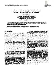
Sapphire crystal growth with heat exchanger method is schematized in Figure 1. The process takes place in an isolated chamber filled with inert gas. Due to high temperatures involved (over 2000C) radiative heat transfer is predominant in the gas. As our focus here is primarily in the prediction of thermally induced stresses in the crystal we will focus on modeling the crystal and assume its thermal environment known. By simple estimation it can be concluded that the role of gravitation (self weight and related forces against supporting surfaces) is 1

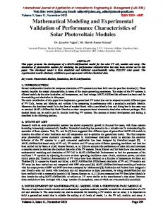
Figure 1: Sapphire Crystal Growth by Heat Exchanger Method (HEM). quite minor compared to expected level of thermal stresses. This, together with the fact that sapphire shrinks during the cooling faster than the supporting materials, enables us to ignore also the surrounding vessel from mechanical considerations. Hence the modeling can be restricted to sapphire alone. The modeled sapphire crystal is sketched in Figure 2. It has three regions: the seed crystal, the expanding cone and the cylindrical part that will be the actual produced crystal to be processed further. In what follows we briefly summarize the governing equations with focus on the material characteristic properties, sketch the simulation scenarios and summarize the main findings. Sample numerical data/graphs are included as appendix. Additional information related to the topic can be found in [Buchanan, 2000], [Chen et al., 2014], [Dobrovinskaya et al., 2009] and [Fang et al., 2013].

2

2

Governing equations

2.1

Heat transfer in solids

Modeling the heat transfer in solids, we have used the following representation ⇢Cp

@T = r · (krT ) @t

(1)

where Cp denotes the heat capacity (constant in our study), k the heat conductivity (likewise treated as constant and isotropic in our study) and T is temperature. We have assumed that system can be controlled outside using heaters so that boundary conditions in producing chamber can be considered thermally insulated. The equation for thermal insulation is defined as (2)

n · ( krT ) = 0

The computations have been executed for two separate boundary conditions for cooling, heat flux and constant out-flow. However, we have reported only the results from out-flow condition. The equation for heat flux boundary condition is described as follows n · ( krT ) = h · (Text

T)

(3)

and boundary conditions for constant out-flow can be represented as n · ( krT ) = q0 .

(4)

Text is external temperature and we have assumed that to be 273K.

2.2

Solid mechanics

Modeling of mechanical deformation and stress analysis, we have considered the following equation r · + Fv = 0 (5) in the domain ⌦. F v stands for volumetric force (gravitation) that is ignored in our study. One-side coupling with thermal effects is done by using following condition = C : (✏ ✏T ) (6) where ⌘ 1⇣ T ru + (ru) and ✏T = ↵(T Tref ). (7) 2 and ↵ denotes the (matrix of) heat expansion coefficients that is slightly anisotropic in our case. Our aim was to disturb the stresses of the system as little as possible using prescribed displacement and other constraints that are necessary for numerical convergence. In particular, we have used spring foundation approach where we ✏=

3

have defined very weak springs in the upper corners of the domain ⌦. Line conditions for spring foundation can be expressed as ·n=

kA (u

(8)

u0 )

where kA is spring constant per unit area. The anisotropic elastic properties are expressed in matrix notation, also called Voigt notation. To do this we take advantage of the symmetry of the stress and strain tensors and express them as six-dimensional vectors in an orthonormal coordinate system (e1, e2, e3) as ⇥ ⇤ ⇥ ⇤ [ ] = 11 , 22 33 , 23 , 13 , 12 ⌘ 1 , 2 , 3 , 4 , 5 , 6 (9) and

⇥ ⇤ ⇥ ⇤ [✏] = ✏11 , ✏22 , ✏33 , 2✏23 , 2✏13 , 2✏12 ⌘ ✏1 , ✏2 ✏3 , ✏4 , ✏5 , ✏6

Then the stiffness tensor Ccan be 2 c1111 c1122 6 c2211 c2222 6 6 c3311 c3322 C=6 6 c2311 c2322 6 4 c3111 c3122 c1211 c1222

(10)

expressed as c1133 c2233 c3333 c2333 c3133 c1233

c1123 c2223 c3323 c2323 c3123 c1223

c1131 c2231 c3331 c2331 c3131 c1231

c1112 c2212 c3312 c2312 c3112 c1212

3

7 7 7 7. 7 7 5

(11)

Sapphire is transversely isotropic material. That is, it is symmetric with respect to a rotation about an axis of symmetry. For such a material, if e3 is the axis of symmetry, Hooke’s law can be expressed as 2 6 6 6 6 6 6 4

1 2 3 4 5 6

3

2

7 6 7 6 7 6 7=6 7 6 7 6 5 6 4

C11 C12 C13 0 0

C12 C11 C13 0 0

C13 C13 C33 0 0

0 0 0 C44 0

0 0 0 0 C44

0

0

0

0

0

32

0 0 0 0 0 1 (C11 2

C12 )

76 76 76 76 76 76 74 5

✏1 ✏2 ✏3 ✏4 ✏5 ✏6

3 7 7 7 7 7 7 5

(12)

For our analysis we split C to isotropic part C iso and anisotropic C an for which an C33 =C33 -C11 an C13 =C13 -C12 and

(13)

an C44 =C44 -C66.

This allows convenient parametrization of the level of anisotropy as C(⌧ ) = C

iso

4

+ ⌧ C an .

(14)

Similar anisotropy is present also in the thermal expansion that differs in e3 -direction from the others. an For Sapphire the main anisotropy relates to C13 that is about 25% of the corresponding isotropic value. For other components of C the anisotropic effects are smaller. Transversely isotropic material allows axisymmetric treatment only if the axis of symmetry and the axis of anisotropy coincide. Otherwise a non axisymmetric effect appears even if all the loading is axisymmetric. To estimate the significance of this effect we have to consider the change in material properties expressed in the axisymmetric frame when the plane of isotropy is tilted by angle ✓. The components of the stiffness tensor in the rotated configuration are related to the components in the reference configuration by the relation cpqrs = lpi lqj lrk lsl cijkl

(15)

where lab are the components of an orthogonal rotation matrix [L(✓)]. Tilting of the material can be modeled by rotation in, say yz-plane. By definition the rotation leaves isotropic properties intact and for the considered anisotropic part the leading order of changes is sin(✓) sin(✓) for small values of ✓. Hence for relatively small rotations the axisymmetric approximation can still be used quite safely.

2.3

Simulated scenarios

We first simulate the system in axisymmetric setting. The material is initially at constant temperature (2000C) and will be cooled with constant rate either from the seed crystal boundaries only or from seed crystal and the conical surface with controlled distribution of heat fluxes simulation parameter. Other boundaries are taken as thermally insulated. For the mechanical part the system is fixed with very weak springs from the boundaries of the uppermost surface to avoid artificial fixture induced stresses in the thermally loaded zone. It should be noted that any kind of support of the seed crystal (fixing either the z-displacements or all displacements at the lowermost surface) leads to stress peaks at the fixed boundary. The following scenarios were simulated: • equal cooling power to seed crystal and cone – isotropic material – anisotropic material • 75% of cooling to seed crystal, 25 % to cone surface – isotropic material – anisotropic material

5

Figure 2: Geometry and mesh used in computations. The temperature histories were the same for all comparable cases as the temperature evolution does not depend on mechanical deformations (in our simplified model) and hence presented only once. Between the scenarios we compared the following quantities: • peak stress • stress distribution in the symmetry plane • stress distribution on the surface • distribution of total displacement All these were evaluated after 3600 s of cooling. Moreover the evolution of temperature and stress on the symmetry axis was monitored for longer time. For 3D simulations the above scenarios were repeated and in addition we monitored stress distribution in a cross section and minima and maxima of stresses on the circumference as indicator of the numerics induced loss of symmetry. Finally for both cooling scenarios the 3D simulation was done for anisotropic material that was rotated 90 degrees (changing y- and z- coordinates).

3

Numerical considerations

Figure 2 presents the used geometries and defined mesh for the computations. Numerical results have been simulated using Comsol Multiphysics software and many of the predefined configurations have been used. Meshes have been build using definition ”finer” and solver configuration have been accepted as it is by default. Computational time used in axi-symmetrical setup was around 20 s and full 3D computing takes time approximately 10 minutes. Some of the used parameters are represented in the table 1.

6

Property Density Thermal conductivity Coefficient of the thermal expansion Heat capacity at constant pressure

Name ⇢ k ↵ Cp

7

Value 3980 35 8 · 10E 800

6

Unit kg/m3 W/(m · K) 1/K J/(kg/K)

Table 1: Material parameters.

4

Analysis of the results and conclusions

We have presented the main results in the Table 2. In our experiments we found up to 8% difference in the stress peak between isotropic and anisotropic material models. As a summary we can conclude that anisotropic material model should be used. If the material is aligned with the symmetry axis, the simulation can be easily done with axisymmetric model. In the full 3D-model we noticed that the grid effects cause artificial asymmetry and hide the anisotropic effects partially. As a whole 3D simulation would require quite fine grid to be able to give reliable results. The results depend, naturally, quite strongly on the boundary conditions. More information of actual cooling strategies would be needed. The simulated scenarios are quite extreme in that respect concentrating the heat flux to a small part of the crystal boundary. More even distribution of heat flux is likely to produce lower peak stresses. Due to strong shrinking of sapphire even minor blocking of deformations induces significant stresses. Hence for realistic modeling the supports and contact to them must be modeled carefully (contact surfaces allowing detachment during shrinking). Situations where the material anisotropy is not aligned with symmetry axis were studied in two ways. Numerically we studied the case where crystal is turned 90 degrees. In this case clear symmetry loss was anticipated. We noticed over20% asymmetry in peak stresses and higher Von Mises stress levels. For small deviations between the material and symmetry axes we concluded with sketchy perturbation analysis that for small rotations loss of symmetry is proportional to sin2 . Hence, given the challenges in 3D simulations, it may be more reliable to use anisotropic axisymmetric model even if the positioning of the seed crystal and its orientation are not perfect. As a summary of conclusions is that material anisotropy should be taken into the model. It has 10% effect to z-displacements and may effect simulations with realistic supporting mechanisms. Moreover, it effects to peak stresses. Material anisotropy can be implemented in axisymmetric code and it is not overly sensitive to perfect alignment to symmetry axis. However, there is no immediate need for 3D model. First of all, it is costly compared to axisymmetric model is same level of reliability is aimed to. Secondly, there are no dominant 3D effects present in the system apart from growing in ”wrong” direction or from Grasshoff convection in melt phase. 7

Simulation Axisymmetric Axisymmetric Axisymmetric Axisymmetric 3D 3D 3D 3D

Cooling 50 50 75 75 50 50 75 75

Isotropy Isotropic Anisotropic Isotropic Anisotropic Isotropic Anisotropic Isotropic Anisotropic

Peak stress 3,07E+07 3,05E+07 4,72E+07 4,71E+07 3,51E+07 3,25E+07 5,36E+07 4,97E+07

Displacement 1,16E-04 1,26E-04 1,41E-04 1,52E-04 1,21E-04 1,32E-04 1,47E-04 1,57E-04

Table 2: Peak stresses and displacements.

5

Discussion

Because this was small workshop research related to event of mathematical modeling of industrial problems, it is convenient to express some notes about the our modeling process. At the first, we focused on the question of comparison between axisymmetric and full 3D computations. The starting point was 3D simulation of thermal expansion induced stresses. Using extreme scenarios, we estimate the role of the (asymmetric) anisotropy. The lack of practical knowledge of the dimensions of real system drives us to working with world record scale dimensions. Next, we build up axisymmetric model with smaller dimensions. After some analytical approximations, we succeeded to estimate semi-realistic parameters to heat flows etc. Practically the estimation relies on the information that the product took one week time to cool down. In the workshop, we had limited time resources, and therefore some details are excluded from this report.

8

References [Buchanan, 2000] Buchanan, G. R. (2000). Vibration of truncated conical cylinders of crystal class 6/mmm. Journal of Vibration and Control, 6(7), 985–998. [Chen et al., 2014] Chen, C.-H., Chen, J.-C., Chiue, Y.-S., Chang, C.-H., Liu, C.-M., & Chen, C.-Y. (2014). Thermal and stress distributions in larger sapphire crystals during the cooling process in a kyropoulos furnace. Journal of Crystal Growth, 385, 55–60. [Dobrovinskaya et al., 2009] Dobrovinskaya, E. R., Lytvynov, L. A., & Pishchik, V. (2009). Sapphire: material, manufacturing, applications. Springer Science & Business Media. [Fang et al., 2013] Fang, H., Pan, Y., Zheng, L., Zhang, Q., Wang, S., & Jin, Z. (2013). To investigate interface shape and thermal stress during sapphire single crystal growth by the cz method. Journal of Crystal Growth, 363, 25–32.

9

APPENDIX Temperature

Figure 3: Temperature fields using full 3D computations. Surface and cut-plane. 50/50 cooling.

10

Figure 4: Temperature evolution versus time. The behavior will be similar until the end. 50/50 and 75/25 cooling.

11

Figure 5: Temperature fields in surface and cut-off plane using full 3D computations. 25/75 cooling.

12

Von Mises Stress

Figure 6: Isotropic and anisotropic Von Mises stress fields using axial symmetric approach. 50/50 cooling.

13

Figure 7: Isotropic and anisotropic Von Mises stress fields using axial symmetric approach, 3D-view. 50/50 cooling.

14

Figure 8: Isotropic and anisotropic Von Mises stress fields using full 3D computations. 50/50 cooling.

15

Figure 9: Isotropic and anisotropic Von Mises stress fields in cut-off plane using full 3D computations. 50/50 cooling.

16

Figure 10: Isotropic and anisotropic Von Mises stress fields using axial symmetric approach. 25/75 cooling. 17

Figure 11: Isotropic and anisotropic Von Mises stress fields using axial symmetric approach, 3D-view. 25/75 cooling.

18

Figure 12: Isotropic and anisotropic Von Mises stress fields using full 3D computations. 25/75 cooling.

19

Figure 13: Isotropic and anisotropic Von Mises stress fields in cut-off plane using full 3D computations. 25/75 cooling.

20

Figure 14: Asymmetric and symmetric anisotropic Von Mises stress fields using full 3D computations. 25/75 cooling.

21

Figure 15: Asymmetric and symmetric anisotropic Von Mises stress fields in cut-off plane using full 3D computations. 25/75 cooling.

22

Figure 16: Asymmetric anisotropicVon Mises stress fields using full 3D computations. 75/25 and 50/50 cooling.

23

Figure 17: Asymmetric anisotropic Von Mises stress fields in cut-off plane using full 3D computations. 75/25 and 50/50 cooling.

24

Figure 18: asymmetric and symmetric anisotropic Von Mises stress cut using full 3D computations.

25

Displacement

Figure 19: Isotropic and anisotropic displacement fields using axial symmetric approach. 50/50 cooling.

26

Figure 20: Isotropic and anisotropic displacements using full 3D computations. 50/50 cooling.

27

Figure 21: Isotropic and anisotropic displacement fields using axial symmetric approach. 25/75 cooling.

28

Figure 22: Isotropic and anisotropic displacements using full 3D computations. 25/75 cooling.

29

Figure 23: Asymmetric and symmetric anisotropic displacements using full 3D computations. 25/75 cooling.

30

Figure 24: Asymmetric anisotropic displacements using full 3D computations. 75/25 and 50/50 cooling.

31

Evolutionary behavior

Figure 25: Isotropic and anisotropic Von Mises stress evolution in the middle line of the system using full 3D computations. 50/50 cooling.

32

Figure 26: Isotropic and anisotropic Von Mises stress evolution in the middle line of the system using full 3D computations. 25/75 cooling.

33

Figure 27: Asymmetric and symmetric anisotropic Von Mises stress evolution in the middle line of the system using full 3D computations. 25/75 cooling.

34

Figure 28: Asymmetric anisotropic Von Mises stress evolution in the middle line of the system using full 3D computations. 75/25 and 50/50 cooling.

35