for a structure of n nodes, the global stiffness matrix KG will be a matrix ... Interval Finite Element Method with MATLAB. ® ...... tetrahedral (solid) element having.
CHAPTER 9
MATLAB® Code for Three-Dimensional Interval Finite Element In this chapter, we will develop the MATLAB® codes for three-dimensional interval finite element, viz. that of space truss, space frame, and linear tetrahedral elements. A systematic procedure is again followed to develop the MATLAB® codes. A set of MATLAB® functions are created first, and then these are executed to investigate few example problems.
9.1 MATLAB® CODE FOR SPACE TRUSS ELEMENT The space truss element is a three-dimensional finite element that is characterized by linear shape functions. Each space truss element has six degrees of freedom where each node contributes three degrees of freedom. Hence, for a structure of n nodes, the global stiffness matrix KG will be a matrix of size 3n � 3n. Consider a space truss element with interval modulus of elasticity EI, cross-sectional area A, and length l. The inclined space truss element makes angles θx, θy, and θz with the global axes x, y, and z, respectively. For simplicity, the interval modulus of elasticity EI is written next as E only. As discussed in previous chapters, the interval modulus of elasticity E is defined again as E I ¼ ½a, b� ¼ E ¼ a + w ½0, 1�
(9.1)
where a and b are the left and the right bounds of the interval modulus of elasticity E; w ¼ b � a is the width of the interval. Interval (Eq. 9.1) can be represented in the parametric form E ¼ a + wα
(9.2)
where α ¼ [0, 1]. This generic form is used in further discussion. The interval elemental stiffness matrix for space truss element may be given from Eq. (8.15) Interval Finite Element Method with MATLAB® https://doi.org/10.1016/B978-0-12-812973-9.00009-6
© 2018 Elsevier Inc. All rights reserved.
119
Interval Finite Element Method with MATLAB®
120
2
Cx2
Cx Cy
Cx Cz
�Cx2
�Cx Cy �Cx Cz
3
6 7 Cy2 Cy Cz �Cy Cx �Cy2 �Cy Cz 7 6 Cy Cx 6 7 Cz2 �Cz Cx �Cz Cy �Cz2 7 EA 6 6 Cz Cx Cz Cy 7 ½K � ¼ 6 7 (9.3) 2 7 l 6 �Cx2 �Cx Cy �Cx Cz C C C C C x y x z x 6 7 6 �C C �Cy2 �Cy Cz Cy Cx Cy2 Cy Cz 7 y x 4 5 2 2 �Cz Cx �Cz Cy �Cz Cz Cx Cz Cy Cz Since the space truss element has six degrees of freedom, the interval elemental stiffness matrix is of order 6 � 6. Hence, for a system of n � 1 elements (n nodes), the size of the global stiffness matrix KG will be of order 3n � 3n. Here, the global stiffness matrix KG is obtained by assembling the element stiffness matrices Ki , i ¼ 1 , 2 , … , n, using the developed procedure in MATLAB® function named as SpaceTrussElementAssemble.m. After the formation of global stiffness matrix KG, we get the following system of equations ½KG�fU g ¼ fF g
(9.4)
where U and F are called the global nodal displacement and the global nodal force vectors, respectively. Next, the boundary conditions are implemented to the vectors U and F, and Eq. (9.4) may be solved by any standard methods for the system of equations. In the following, we will discuss various MATLAB® functions developed for the space truss element (Kattan, 2007; Nayak and Chakraverty, 2014).
9.1.1 MATLAB® Functions for Space Truss Element 1. SpaceTrussElementLength (x1, y1, z1, x2, y2, z2) This MATLAB® function calculates the length of the space truss element that has the first node at (x1, y1, z1) and second node at (x2, y2, z2). It returns a crisp real value. function y = SpaceTrussElementLength (x1, y1, z1, x2, y2, z2) % SpaceTrussElementLength
This function gives length of the space
%
truss element whose first and second have
%
coordinates (x1,y1,z1) and (x2,y2,z2)
%
respectively.
y= sqrt((x2-x1)^2 +(y2-y1)^2 +(z2-z1)^2);
MATLAB® Code for Three-Dimensional Interval Finite Element
121
2. SpaceTrussElementStiffness (a, b, alpha, A, l, thetax, thetay, thetaz) This MATLAB® function calculates the element stiffness matrix K for each space truss element having interval modulus of elasticity E, cross-section area A, length l, and angles thetax, thetay, and thetaz (in degrees). Here, a and b are the left and the right bounds of interval modulus of elasticity and alpha belongs to [0, 1]. It gives element stiffness for plane truss element of size 6 � 6. function y=SpaceTrussElementStiffness (a,b,alpha,E,A,L,thetax, thetay,thetaz) % SpaceTrussElementStiffness
This function gives element stiffness
%
matrix for a space truss element having
%
modulus of elasticity E, cross sectional
%
area A, length L and angles thetax,
%
thetay, thetaz (in degrees). Here, a
%
and b are the left and right bounds of
%
interval modulus of elasticity; alpha
%
belongs to [0, 1].
E=a +(b-a)*alpha; x=thetax*pi/180; u=thetay*pi/180; v=thetaz*pi/180; Cx=cos(x); Cy=cos(u); Cz=cos(v); w=[Cx^2 Cx*Cy Cx*Cz;Cx*Cy Cy^2 Cy*Cz;Cx*Cz Cy*Cz Cz^2]; y=(E*A/L)*[w -w;-w w];
3. SpaceTrussElementAssemble (KG, K, i, j) The titled MATLAB® function is used to assemble the elemental stiffness matrix K of the space truss element whose nodes are i (left-end node) and j (right-end node) into the global stiffness matrix KG. It gives 3n � 3n global stiffness matrix KG. function y = SpaceTrussElementAssemble (KG, K, i, j) % SpaceTrussElementAssemble
This function is used to assemble the
%
element stiffness matrix K of the space
%
truss element having nodes i and j into the
%
global stiffness matrix KG.
KG(3*i-2,3*i-2)=KG(3*i-2,3*i-2)+K(1,1); KG(3*i-2,3*i-1)=KG(3*i-2,3*i-1)+K(1,2); KG(3*i-2,3*i)=KG(3*i-2,3*i)+K(1,3); KG(3*i-2,3*j-2)=KG(3*i-2,3*j-2)+K(1,4);
Interval Finite Element Method with MATLAB®
122
KG(3*i-2,3*j-1)=KG(3*i-2,3*j-1)+K(1,5); KG(3*i-2,3*j)=KG(3*i-2,3*j)+K(1,6); KG(3*i-1,3*i-2)=KG(3*i-1,3*i-2)+K(2,1); KG(3*i-1,3*i-1)=KG(3*i-1,3*i-1)+K(2,2); KG(3*i-1,3*i)=KG(3*i-1,3*i)+K(2,3); KG(3*i-1,3*j-2)=KG(3*i-1,3*j-2)+K(2,4); KG(3*i-1,3*j-1)=KG(3*i-1,3*j-1)+K(2,5); KG(3*i-1,3*j)=KG(3*i-1,3*j)+K(2,6); KG(3*i,3*i-2)=KG(3*i,3*i-2)+K(3,1); KG(3*i,3*i-1)=KG(3*i,3*i-1)+K(3,2); KG(3*i,3*i)=KG(3*i,3*i)+K(3,3); KG(3*i,3*j-2)=KG(3*i,3*j-2)+K(3,4); KG(3*i,3*j-1)=KG(3*i,3*j-1)+K(3,5); KG(3*i,3*j)=KG(3*i,3*j)+K(3,6); KG(3*j-2,3*i-2)=KG(3*j-2,3*i-2)+K(4,1); KG(3*j-2,3*i-1)=KG(3*j-2,3*i-1)+K(4,2); KG(3*j-2,3*i)=KG(3*j-2,3*i)+K(4,3); KG(3*j-2,3*j-2)=KG(3*j-2,3*j-2)+K(4,4); KG(3*j-2,3*j-1)=KG(3*j-2,3*j-1)+K(4,5); KG(3*j-2,3*j)=KG(3*j-2,3*j)+K(4,6); KG(3*j-1,3*i-2)=KG(3*j-1,3*i-2)+K(5,1); KG(3*j-1,3*i-1)=KG(3*j-1,3*i-1)+K(5,2); KG(3*j-1,3*i)=KG(3*j-1,3*i)+K(5,3); KG(3*j-1,3*j-2)=KG(3*j-1,3*j-2)+K(5,4); KG(3*j-1,3*j-1)=KG(3*j-1,3*j-1)+K(5,5); KG(3*j-1,3*j)=KG(3*j-1,3*j)+K(5,6); KG(3*j,3*i-2)=KG(3*j,3*i-2)+K(6,1); KG(3*j,3*i-1)=KG(3*j,3*i-1)+K(6,2); KG(3*j,3*i)=KG(3*j,3*i)+K(6,3); KG(3*j,3*j-2)=KG(3*j,3*j-2)+K(6,4); KG(3*j,3*j-1)=KG(3*j,3*j-1)+K(6,5); KG(3*j,3*j)=KG(3*j,3*j)+K(6,6); y= KG;
4. SpaceTrusssElementForce (a, b, alpha, A, l, thetax, thetay, thetaz, u) This MATLAB® function is used to calculate the element force vector, which returns 6 � 1 vector. function y=SpaceTrusssElementForce (a,b,alpha,A,l,thetax,thetay, thetaz,u) % SpaceTrusssElementForce
This function gives element force when
%
the modulus of elasticity E, the cross
MATLAB® Code for Three-Dimensional Interval Finite Element
123
%
sectional area A, length l, the angles
%
thetax, thetay, thetaz (in degrees)
%
and the element nodal displacement vector
%
u are given.
E=a +(b-a)*alpha; x=thetax*pi/180; v=thetay*pi/180; w=thetaz*pi/180; Cx=cos(x); Cy=cos(v); Cz=cos(w); y=(E*A/l)*[-Cx -Cy -Cz Cx Cy Cz]*u;
Let us now introduce the algorithm to write the program of space truss element using these MATLAB® functions. Step 1: Discretization of the domain The domain is discretized into a finite number of elements. Then, the element connectivity table is obtained. Step 2: Evaluation of element stiffness matrices Element stiffness matrices Ki , i ¼ 1 , 2 , … , n are generated by using the MATLAB® function “SpaceTrussElementStiffness.” Here, each matrix has size 4 � 4. Step 3: Evaluation of global stiffness matrix Element stiffness matrices are assembled by using the MATLAB® function “SpaceTrussElementAssemble” and global stiffness matrix is formed. Step 4: Application of boundary conditions Boundary conditions are applied to the global stiffness matrix and a global system of equations are obtained. Step 5: Solution of system of equations A system of equations (after applying boundary conditions to the global system of equations) are solved. The unknown variables are found by using the MATLAB® function “SpaceTrussElementForces.”
Example 9.1 Consider a system of space truss elements shown in Fig. 9.1. Here, the system is supported with ball and socket joints at nodes 1, 2, and 3, which allow rotations but no translation. The interval modulus of elasticity is E ¼ [200, 220] GPa; area of element 1, 2, and 3 are A14 ¼ 0.002 m2, A24 ¼ 0.003 m2, A34 ¼ 0.002 m2, respectively; and the
124
Interval Finite Element Method with MATLAB®
Fig. 9.1 System of space truss elements.
Table 9.1 Element connectivity for system of space truss elements Element number Node i Node j
1 2 3
1 2 3
4 4 4
external force P ¼ 10 kN is at node 4 along directions 1 to 4. We will determine the displacements at each node. The system of space truss elements (Fig. 9.1) is composed of three space truss elements where each element has a common node, i.e., node 4. Considering the discretization of the system of space trusses, the element connectivity is presented in Table 9.1. In this table, the nodes i and j represent the first and the last nodes of the element. In Fig. 9.1, the first node (node 1), second node (node 2), and third node (node 3) are fixed; hence, the displacement at nodes 1, 2, and 3 is zero. However, a force P ¼ 10 kN is applied at the node 4. Next, we will investigate the nodal displacements. Considering the architecture of the space truss elements and these MATLAB® functions, Code 9.1 is developed to investigate the displacements. Code 9.1 is developed for the alpha (α) value of zero only.
Code 9.1: Space Truss Element A1= 0.002; A2= 0.003; A3= 0.002; l1= SpaceTrussElementLength (0, 0, -3, 0, 5, 0);
MATLAB® Code for Three-Dimensional Interval Finite Element
125
l2=SpaceTrussElementLength (-4, 0, 0, 0, 5, 0); l3=SpaceTrussElementLength (0, 0, 3, 0, 5, 0); theta1x= acos(0/l1)*(180/pi); theta1y= acos(5/l1)*(180/pi); theta1z= acos(3/l1)*(180/pi); theta2x= acos(4/l2)*(180/pi); theta2y= acos(5/l2)*(180/pi); theta2z= acos(0/l2)*(180/pi); theta3x= acos(0/l3)*(180/pi); theta3y= acos(5/l3)*(180/pi); theta3z= acos(-3/l3)*(180/pi); %----------------------% Stiffness matrices of the elements %----------------------K1=SpaceTrussElementStiffness(200,220,0,A1,l1,theta1x, theta1y,theta1z); K2=SpaceTrussElementStiffness(200,220,0,A2,l2,theta2x, theta2y,theta2z); K3=SpaceTrussElementStiffness(200,220,0,A3,l3,theta3x, theta3y,theta3z); %----------------------% Assembling of the stiffness matrices %----------------------KG=zeros(12,12); KG=SpaceTrussElementAssemble(KG, K1, 1, 4); KG=SpaceTrussElementAssemble(KG, K2, 2, 4); KG=SpaceTrussElementAssemble(KG, K3, 3, 4); %- - - - - - - - - - - - - - - - - - - - - - - %Boundary conditions %- - - - - - - - - - - - - - - - - - - - - - - K=[KG(10:12,10:12)]; f=[10;0;0]; %----------------------% Nodal displacements %----------------------u=inv(K)*f
Using Code 9.1 for different values of alpha (α), nodal displacements for this system of space trusses are obtained. The nodal displacements are given in Table 9.2. The union of these displacements generates the united solution (displacements) of the system.
126
Interval Finite Element Method with MATLAB®
Table 9.2 Nodal displacements of system of space truss elements for different α values α50 α 5 0.2 α 5 0.4 α 5 0.6 α 5 0.8 α51
u10 u11 u12
0.4284 �10�3 �0.1239 �10�3 �0.0000 �10�3
0.4200 �10�3 �0.1215 �10�3 �0.0000 �10�3
0.4119 �10�3 �0.1191 �10�3 �0.0000 �10�3
0.4041 �10�3 �0.1169 �10�3 �0.0000 �10�3
0.3966 �10�3 �0.1147 �10�3 �0.0000 �10�3
0.3894 �10�3 �0.1126 �10�3 0.0000 �10�3
Table 9.3 United solution for space truss system
u10 u11 u12
[0.3894, 0.4284] � 10�3 [�0.1239, �0.1126] � 10�3 [0, 0]
Considering the various displacements in Table 9.2, we get the interval solution (united solution) that is presented in Table 9.3.
9.2 MATLAB® CODE FOR SPACE FRAME ELEMENT Space frame element is a three-dimensional finite element. It is similar to the beam element in addition to two extra properties, i.e., it experiences an axial force due to loads and these elements are oriented in any direction in the plane. Each beam element has interval modulus of elasticity EI, length l, cross-sectional area A, moment of inertia Iy and Iz, and polar moment of inertia J. Each plane frame element has two nodes that make angles θx, θy, and θz (in degrees) with global axes X, Y, and Z, respectively, in counterclockwise direction. Here, for simplicity, the interval modulus of elasticity EI is considered as E. The interval modulus of elasticity E and its parametric form are defined in Eqs. (9.1), (9.2), respectively. As the space frame undergoes both the axial and the transversal forces, it has twelve degrees of freedom (six degrees of freedom at each node). The element stiffness matrix for beam element in space is from Eq. (8.30)
2
MATLAB® Code for Three-Dimensional Interval Finite Element
3 EI A EI A 0 0 0 0 0 � 0 0 0 0 0 7 6 l l 6 7 I I I 12E Iz 6E Iz 12E Iz 6EI Iz 7 6 6 0 7 0 0 0 0 � 3 0 0 0 6 l3 l2 l l2 7 6 7 I I I I 12E Iy 6E Iy 12E Iy 6E Iy 6 7 0 0 � 0 0 0 � 0 � 0 6 0 7 6 7 l3 l2 l3 l2 6 7 GJ GJ 6 0 7 0 0 0 0 0 � 0 0 0 0 6 7 l l 6 7 I I I I 6 7 6E I 4E I 6E I 2E I y y y y 6 0 0 � 2 0 0 0 0 0 0 7 6 7 2 l l l l 6 7 I I I I 6 6E Iz 4E Iz 6E Iz 2E Iz 7 6 0 7 0 0 0 0 0 0 0 � 6 7 l2 l l2 l ½K � ¼ 6 7 EI A 6 EI A 7 6� 0 0 0 0 0 0 0 0 0 0 7 6 7 l l 6 12E I Iy 12EI Iz 6EI Iz 6EI Iz 7 6 7 � 3 0 0 0 � 2 0 0 0 0 � 2 7 6 0 3 6 l l l l 7 6 7 12E I Iy 6E I Iy 12E I Iy 6E I Iy 6 0 7 0 � 0 0 0 0 0 0 6 7 l3 l2 l3 l2 6 7 6 7 GJ GJ 6 0 0 0 0 0 0 0 0 7 0 0 � 6 7 l l 6 7 6E I Iy 2E I Iy 6E I Iy 4E I Iy 6 7 6 0 7 0 � 2 0 0 0 0 0 0 2 6 7 l l l l 4 6E I Iz 2EI Iz 6EI Iz 4EI Iz 5 0 0 0 0 0 0 0 0 � 2 l2 l l l (9.5)
127
Interval Finite Element Method with MATLAB®
128
The interval elemental stiffness matrix for space frame element is of order 12 � 12, due to the twelve degrees of freedom (six at each nodes). For a structure or a domain with n nodes, we obtain a global stiffness matrix KG of size 6n � 6n. The elemental stiffness matrices are assembled through the MATLAB® function. SpaceFrameElementAssemble.m and global stiffness matrix KG is obtained. Considering the global stiffness matrix along with the global displacement vectors and global force vectors, we get the global elemental equation (9.4). Finally, the boundary conditions are applied to Eq. (9.4) and unknown field variables may be obtained by using standard methods for the system of equations. Next, we will discuss various MATLAB® functions developed for the space frame element (Chapman, 2007; Nayak and Chakraverty, 2014).
9.2.1 MATLAB® Functions for Space Frame Element 1. SpaceFrameElementLength (x1, y1, z1, x2, y2, z2) This MATLAB® function calculates the length of the space frame element that has the first node at (x1, y1, z1) and the second node at (x2, y2, z2). It returns a crisp real value. function y = SpaceFrameElementLength (x1,y1,z1,x2,y2,z2) % SpaceFrameElementLength
This function gives length of the space
%
frame element whose first and second
%
nodes have coordinates (x1,y1,z1) and
%
(x2,y2,z2) respectively.
y= sqrt((x2-x1)^2 +(y2-y1)^2 +(z2-z1)^2);
2. SpaceFrameElementStiffness (a, b, alpha, G, A, Iy, Iz, J, x1, y1, z1, x2, y2, z2) This MATLAB® function calculates the element stiffness matrix K for each space frame element with interval modulus of elasticity E, length l, crosssectional area A, moment of inertia Iy and Iz, polar moment of inertia J, and angles θx, θy, and θz (in degrees) with global axes x, y, and z, respectively, in counterclockwise direction. Here, a and b are the left and the right bounds of interval modulus of elasticity and alpha belongs to [0, 1]. It gives the element stiffness matrix for space frame element of size 12 � 12. function y=SpaceFrameElementStiffness (a,b,alpha,G,A,Iy,Iz,J,x1,y1,z1,x2,y2,z2) % SpaceFrameElementStiffness
This function gives element stiffness
%
matrix for a space frame element having
%
interval modulus of elasticity E, shear
MATLAB® Code for Three-Dimensional Interval Finite Element
129
%
modulus of elasticity G, cross sectional
%
area A, moments of inertia Iy and Iz,
%
torsional constant J, coordinates
%
(x1,y1,z1) for the first node and
%
coordinates (x2,y2,z2) for the second
%
node. Here, a and b are the left and right
%
bounds of interval modulus of elasticity;
%
alpha belongs to [0, 1].
E=a +(b-a)*alpha; L=sqrt((x2-x1)^2+(y2-y1)^2+(z2-z1)^2); w1 =E*A/L; w2 =12*E*Iz/(L^3); w3 =6*E*Iz/(L^2); w4 =4*E*Iz/L; w5 =2*E*Iz/L; w6 =12*E*Iy/(L^3); w7 =6*E*Iy/(L^2); w8 =4*E*Iy/L; w9 =2*E*Iy/L; w10=G*J/L; Kprime=[w1 0 0 0 0 0 -w1 0 0 0 0 0; 0 w2 0 0 0 w3 0 -w2 0 0 0 w3; 0 0 w6 0 -w7 0 0 0 -w6 0 -w7 0; 0 0 0 w10 0 0 0 0 0 -w10 0 0; 0 0 -w7 0 w8 0 0 0 w7 0 w9 0; 0 w3 0 0 0 w4 0 -w3 0 0 0 w5; -w1 0 0 0 0 0 w1 0 0 0 0 0; 0 -w2 0 0 0 -w3 0 w2 0 0 0 -w3; 0 0 -w6 0 w7 0 0 0 w6 0 w7 0; 0 0 0 -w10 0 0 0 0 0 w10 0 0; 0 0 -w7 0 w9 0 0 0 w7 0 w8 0; 0 w3 0 0 0 w5 0 -w3 0 0 0 w4]; if x1==x2 & y1==y2 if z2> z1 Lambda=[0 0 1;0 1 0;-1 0 0]; else Lambda=[0 0 -1;0 1 0;1 0 0]; end
Interval Finite Element Method with MATLAB®
130
else CXx=(x2-x1)/L; CYx=(y2-y1)/L; CZx=(z2-z1)/L; D=sqrt(CXx^2+ CYx^2); CXy=-CXx/D; CYy= CXx/D; CZy= 0; CXz=-CXx*CZx/D; CYz=-CYx*CZx/D; CZz= D; Lambda=[CXx CYx CZx; CXy CYy CZy; CXz CYz CZz]; end R =[Lambda zeros(3,3) zeros(3,3) zeros(3,3);zeros(3,3) Lambda zeros (3,3) zeros(3,3);zeros(3,3) zeros(3,3) Lambda zeros(3,3);zeros(3,3) zeros(3,3) zeros(3,3) Lambda]; y =R’*Kprime*R;
3. SpaceFrameElementAssemble (KG, K, i, j) The titled MATLAB® function is used to assemble the elemental stiffness matrix K of the space frame element whose nodes are i (left-end node) and j (right-end node) into the global stiffness matrix KG. This function gives 6n � 6n global stiffness matrix KG. function y = SpaceFrameElementAssemble(KG, K, i, j) %SpaceFrameElementAssemble
This function is used to assemble the
%
element stiffness matrix K of the space
%
frame element with nodes i and j into the
%
global stiffness matrix KG.
KG(6*i-5,6*i-5)=KG(6*i-5,6*i-5)+K(1,1); KG(6*i-5,6*i-4)=KG(6*i-5,6*i-4)+K(1,2); KG(6*i-5,6*i-3)=KG(6*i-5,6*i-3)+K(1,3); KG(6*i-5,6*i-2)=KG(6*i-5,6*i-2)+K(1,4); KG(6*i-5,6*i-1)=KG(6*i-5,6*i-1)+K(1,5); KG(6*i-5,6*i)=KG(6*i-5,6*i)+K(1,6); KG(6*i-5,6*j-5)=KG(6*i-5,6*j-5)+K(1,7); KG(6*i-5,6*j-4)=KG(6*i-5,6*j-4)+K(1,8); KG(6*i-5,6*j-3)=KG(6*i-5,6*j-3)+K(1,9); KG(6*i-5,6*j-2)=KG(6*i-5,6*j-2)+K(1,10); KG(6*i-5,6*j-1)=KG(6*i-5,6*j-1)+K(1,11); KG(6*i-5,6*j)=KG(6*i-5,6*j)+K(1,12); KG(6*i-4,6*i-5)=KG(6*i-4,6*i-5)+K(2,1);
MATLAB® Code for Three-Dimensional Interval Finite Element
KG(6*i-4,6*i-4)=KG(6*i-4,6*i-4)+K(2,2); KG(6*i-4,6*i-3)=KG(6*i-4,6*i-3)+K(2,3); KG(6*i-4,6*i-2)=KG(6*i-4,6*i-2)+K(2,4); KG(6*i-4,6*i-1)=KG(6*i-4,6*i-1)+K(2,5); KG(6*i-4,6*i)=KG(6*i-4,6*i)+K(2,6); KG(6*i-4,6*j-5)=KG(6*i-4,6*j-5)+K(2,7); KG(6*i-4,6*j-4)=KG(6*i-4,6*j-4)+K(2,8); KG(6*i-4,6*j-3)=KG(6*i-4,6*j-3)+K(2,9); KG(6*i-4,6*j-2)=KG(6*i-4,6*j-2)+K(2,10); KG(6*i-4,6*j-1)=KG(6*i-4,6*j-1)+K(2,11); KG(6*i-4,6*j)=KG(6*i-4,6*j)+K(2,12); KG(6*i-3,6*i-5)=KG(6*i-3,6*i-5)+K(3,1); KG(6*i-3,6*i-4)=KG(6*i-3,6*i-4)+K(3,2); KG(6*i-3,6*i-3)=KG(6*i-3,6*i-3)+K(3,3); KG(6*i-3,6*i-2)=KG(6*i-3,6*i-2)+K(3,4); KG(6*i-3,6*i-1)=KG(6*i-3,6*i-1)+K(3,5); KG(6*i-3,6*i)=KG(6*i-3,6*i)+K(3,6); KG(6*i-3,6*j-5)=KG(6*i-3,6*j-5)+K(3,7); KG(6*i-3,6*j-4)=KG(6*i-3,6*j-4)+K(3,8); KG(6*i-3,6*j-3)=KG(6*i-3,6*j-3)+K(3,9); KG(6*i-3,6*j-2)=KG(6*i-3,6*j-2)+K(3,10); KG(6*i-3,6*j-1)=KG(6*i-3,6*j-1)+K(3,11); KG(6*i-3,6*j)=KG(6*i-3,6*j)+K(3,12); KG(6*i-2,6*i-5)=KG(6*i-2,6*i-5)+K(4,1); KG(6*i-2,6*i-4)=KG(6*i-2,6*i-4)+K(4,2); KG(6*i-2,6*i-3)=KG(6*i-2,6*i-3)+K(4,3); KG(6*i-2,6*i-2)=KG(6*i-2,6*i-2)+K(4,4); KG(6*i-2,6*i-1)=KG(6*i-2,6*i-1)+K(4,5); KG(6*i-2,6*i)=KG(6*i-2,6*i)+K(4,6); KG(6*i-2,6*j-5)=KG(6*i-2,6*j-5)+K(4,7); KG(6*i-2,6*j-4)=KG(6*i-2,6*j-4)+K(4,8); KG(6*i-2,6*j-3)=KG(6*i-2,6*j-3)+K(4,9); KG(6*i-2,6*j-2)=KG(6*i-2,6*j-2)+K(4,10); KG(6*i-2,6*j-1)=KG(6*i-2,6*j-1)+K(4,11); KG(6*i-2,6*j)=KG(6*i-2,6*j)+K(4,12); KG(6*i-1,6*i-5)=KG(6*i-1,6*i-5)+K(5,1); KG(6*i-1,6*i-4)=KG(6*i-1,6*i-4)+K(5,2); KG(6*i-1,6*i-3)=KG(6*i-1,6*i-3)+K(5,3); KG(6*i-1,6*i-2)=KG(6*i-1,6*i-2)+K(5,4);
131
132
Interval Finite Element Method with MATLAB®
KG(6*i-1,6*i-1)=KG(6*i-1,6*i-1)+K(5,5); KG(6*i-1,6*i)=KG(6*i-1,6*i)+K(5,6); KG(6*i-1,6*j-5)=KG(6*i-1,6*j-5)+K(5,7); KG(6*i-1,6*j-4)=KG(6*i-1,6*j-4)+K(5,8); KG(6*i-1,6*j-3)=KG(6*i-1,6*j-3)+K(5,9); KG(6*i-1,6*j-2)=KG(6*i-1,6*j-2)+K(5,10); KG(6*i-1,6*j-1)=KG(6*i-1,6*j-1)+K(5,11); KG(6*i-1,6*j)=KG(6*i-1,6*j)+K(5,12); KG(6*i,6*i-5)=KG(6*i,6*i-5)+K(6,1); KG(6*i,6*i-4)=KG(6*i,6*i-4)+K(6,2); KG(6*i,6*i-3)=KG(6*i,6*i-3)+K(6,3); KG(6*i,6*i-2)=KG(6*i,6*i-2)+K(6,4); KG(6*i,6*i-1)=KG(6*i,6*i-1)+K(6,5); KG(6*i,6*i)=KG(6*i,6*i)+K(6,6); KG(6*i,6*j-5)=KG(6*i,6*j-5)+K(6,7); KG(6*i,6*j-4)=KG(6*i,6*j-4)+K(6,8); KG(6*i,6*j-3)=KG(6*i,6*j-3)+K(6,9); KG(6*i,6*j-2)=KG(6*i,6*j-2)+K(6,10); KG(6*i,6*j-1)=KG(6*i,6*j-1)+K(6,11); KG(6*i,6*j)=KG(6*i,6*j)+K(6,12); KG(6*j-5,6*i-5)=KG(6*j-5,6*i-5)+K(7,1); KG(6*j-5,6*i-4)=KG(6*j-5,6*i-4)+K(7,2); KG(6*j-5,6*i-3)=KG(6*j-5,6*i-3)+K(7,3); KG(6*j-5,6*i-2)=KG(6*j-5,6*i-2)+K(7,4); KG(6*j-5,6*i-1)=KG(6*j-5,6*i-1)+K(7,5); KG(6*j-5,6*i)=KG(6*j-5,6*i)+K(7,6); KG(6*j-5,6*j-5)=KG(6*j-5,6*j-5)+K(7,7); KG(6*j-5,6*j-4)=KG(6*j-5,6*j-4)+K(7,8); KG(6*j-5,6*j-3)=KG(6*j-5,6*j-3)+K(7,9); KG(6*j-5,6*j-2)=KG(6*j-5,6*j-2)+K(7,10); KG(6*j-5,6*j-1)=KG(6*j-5,6*j-1)+K(7,11); KG(6*j-5,6*j)=KG(6*j-5,6*j)+K(7,12); KG(6*j-4,6*i-5)=KG(6*j-4,6*i-5)+K(8,1); KG(6*j-4,6*i-4)=KG(6*j-4,6*i-4)+K(8,2); KG(6*j-4,6*i-3)=KG(6*j-4,6*i-3)+K(8,3); KG(6*j-4,6*i-2)=KG(6*j-4,6*i-2)+K(8,4); KG(6*j-4,6*i-1)=KG(6*j-4,6*i-1)+K(8,5); KG(6*j-4,6*i)=KG(6*j-4,6*i)+K(8,6); KG(6*j-4,6*j-5)=KG(6*j-4,6*j-5)+K(8,7);
MATLAB® Code for Three-Dimensional Interval Finite Element
KG(6*j-4,6*j-4)=KG(6*j-4,6*j-4)+K(8,8); KG(6*j-4,6*j-3)=KG(6*j-4,6*j-3)+K(8,9); KG(6*j-4,6*j-2)=KG(6*j-4,6*j-2)+K(8,10); KG(6*j-4,6*j-1)=KG(6*j-4,6*j-1)+K(8,11); KG(6*j-4,6*j)=KG(6*j-4,6*j)+K(8,12); KG(6*j-3,6*i-5)=KG(6*j-3,6*i-5)+K(9,1); KG(6*j-3,6*i-4)=KG(6*j-3,6*i-4)+K(9,2); KG(6*j-3,6*i-3)=KG(6*j-3,6*i-3)+K(9,3); KG(6*j-3,6*i-2)=KG(6*j-3,6*i-2)+K(9,4); KG(6*j-3,6*i-1)=KG(6*j-3,6*i-1)+K(9,5); KG(6*j-3,6*i)=KG(6*j-3,6*i)+K(9,6); KG(6*j-3,6*j-5)=KG(6*j-3,6*j-5)+K(9,7); KG(6*j-3,6*j-4)=KG(6*j-3,6*j-4)+K(9,8); KG(6*j-3,6*j-3)=KG(6*j-3,6*j-3)+K(9,9); KG(6*j-3,6*j-2)=KG(6*j-3,6*j-2)+K(9,10); KG(6*j-3,6*j-1)=KG(6*j-3,6*j-1)+K(9,11); KG(6*j-3,6*j)=KG(6*j-3,6*j)+K(9,12); KG(6*j-2,6*i-5)=KG(6*j-2,6*i-5)+K(10,1); KG(6*j-2,6*i-4)=KG(6*j-2,6*i-4)+K(10,2); KG(6*j-2,6*i-3)=KG(6*j-2,6*i-3)+K(10,3); KG(6*j-2,6*i-2)=KG(6*j-2,6*i-2)+K(10,4); KG(6*j-2,6*i-1)=KG(6*j-2,6*i-1)+K(10,5); KG(6*j-2,6*i)=KG(6*j-2,6*i)+K(10,6); KG(6*j-2,6*j-5)=KG(6*j-2,6*j-5)+K(10,7); KG(6*j-2,6*j-4)=KG(6*j-2,6*j-4)+K(10,8); KG(6*j-2,6*j-3)=KG(6*j-2,6*j-3)+K(10,9); KG(6*j-2,6*j-2)=KG(6*j-2,6*j-2)+K(10,10); KG(6*j-2,6*j-1)=KG(6*j-2,6*j-1)+K(10,11); KG(6*j-2,6*j)=KG(6*j-2,6*j)+K(10,12); KG(6*j-1,6*i-5)=KG(6*j-1,6*i-5)+K(11,1); KG(6*j-1,6*i-4)=KG(6*j-1,6*i-4)+K(11,2); KG(6*j-1,6*i-3)=KG(6*j-1,6*i-3)+K(11,3); KG(6*j-1,6*i-2)=KG(6*j-1,6*i-2)+K(11,4); KG(6*j-1,6*i-1)=KG(6*j-1,6*i-1)+K(11,5); KG(6*j-1,6*i)=KG(6*j-1,6*i)+K(11,6); KG(6*j-1,6*j-5)=KG(6*j-1,6*j-5)+K(11,7); KG(6*j-1,6*j-4)=KG(6*j-1,6*j-4)+K(11,8); KG(6*j-1,6*j-3)=KG(6*j-1,6*j-3)+K(11,9); KG(6*j-1,6*j-2)=KG(6*j-1,6*j-2)+K(11,10);
133
Interval Finite Element Method with MATLAB®
134
KG(6*j-1,6*j-1)=KG(6*j-1,6*j-1)+K(11,11); KG(6*j-1,6*j)=KG(6*j-1,6*j)+K(11,12); KG(6*j,6*i-5)=KG(6*j,6*i-5)+K(12,1); KG(6*j,6*i-4)=KG(6*j,6*i-4)+K(12,2); KG(6*j,6*i-3)=KG(6*j,6*i-3)+K(12,3); KG(6*j,6*i-2)=KG(6*j,6*i-2)+K(12,4); KG(6*j,6*i-1)=KG(6*j,6*i-1)+K(12,5); KG(6*j,6*i)=KG(6*j,6*i)+K(12,6); KG(6*j,6*j-5)=KG(6*j,6*j-5)+K(12,7); KG(6*j,6*j-4)=KG(6*j,6*j-4)+K(12,8); KG(6*j,6*j-3)=KG(6*j,6*j-3)+K(12,9); KG(6*j,6*j-2)=KG(6*j,6*j-2)+K(12,10); KG(6*j,6*j-1)=KG(6*j,6*j-1)+K(12,11); KG(6*j,6*j)=KG(6*j,6*j)+K(12,12); y= KG;
4. SpaceFrameElementForces (a, b, alpha, G, A, Iy, Iz, J, x1, y1, z1, x2, y2, z2, u) This MATLAB® function is used to calculate the element force vector. function y=SpaceFrameElementForces (a,b,alpha,G,A,Iy,Iz,J,x1,y1,z1,x2,y2,z2,u) % SpaceFrameElementForces
This function gives element force vector
%
when the modulus of elasticity E, the
%
shear modulus of elasticity G, the cross
%
sectional area A, moments of inertia Iy
%
and Iz, the torsional constant J, the
%
first and second node coordinates
%
(x1,y1,z1) and (x2,y2,z2) along with the
%
element nodal displacement vector u are
%
given.
E= a+(b-a)*alpha; L =sqrt((x2-x1)^2+(y2-y1)^2+(z2-z1)^2); w1 =E*A/L; w2 =12*E*Iz/(L^3); w3 =6*E*Iz/(L^2); w4 =4*E*Iz/L; w5 =2*E*Iz/L; w6 =12*E*Iy/(L^3); w7 =6*E*Iy/(L^2); w8 =4*E*Iy/L;
MATLAB® Code for Three-Dimensional Interval Finite Element
135
w9 =2*E*Iy/L; w10=G*J/L; Kprime=[w1 0 0 0 0 0 -w1 0 0 0 0 0; 0 w2 0 0 0 w3 0 -w2 0 0 0 w3; 0 0 w6 0 -w7 0 0 0 -w6 0 -w7 0; 0 0 0 w10 0 0 0 0 0 -w10 0 0; 0 0 -w7 0 w8 0 0 0 w7 0 w9 0; 0 w3 0 0 0 w4 0 -w3 0 0 0 w5; -w1 0 0 0 0 0 w1 0 0 0 0 0; 0 -w2 0 0 0 -w3 0 w2 0 0 0 -w3; 0 0 -w6 0 w7 0 0 0 w6 0 w7 0; 0 0 0 -w10 0 0 0 0 0 w10 0 0; 0 0 -w7 0 w9 0 0 0 w7 0 w8 0; 0 w3 0 0 0 w5 0 -w3 0 0 0 w4]; if x1==x2 & y1==y2 if Z2> Z1 Lambda=[0 0 1;0 1 0;-1 0 0]; else Lambda=[0 0 -1;0 1 0;1 0 0]; end else CXx=(x2-x1)/L; CYx=(y2-y1)/L; CZx=(z2-z1)/L; D =sqrt(CXx^2+ CYx^2); CXy=-CXx/D; CYy=CXx/D; CZy=0; CXz=-CXx*CZx/D; CYz=-CYx*CZx/D; CZz=D; Lambda=[CXx CYx CZx; CXy CYy CZy; CXz CYz CZz]; end R=[Lambda zeros (3) zeros (3);zeros(3) Lambda zeros(3) zeros(3); zeros(3) zeros(3) Lambda zeros(3);zeros(3) zeros(3) zeros(3) Lambda]; y= Kprime*R*u;
Let us introduce the algorithm to write the program of plane frame element using these MATLAB® functions.
136
Interval Finite Element Method with MATLAB®
Step 1: Discretization of the domain The domain is discretized into a finite number of elements. Then, the element connectivity table is generated. Step 2: Evaluation of element stiffness matrices Element stiffness matrices Ki , i ¼ 1 , 2 , … , n are obtained by using the MATLAB® function “SpaceFrameElementStiffness.” Here, each matrix has size 12 � 12. Step 3: Evaluation of global stiffness matrix Element stiffness matrices are assembled by using the MATLAB® function “SpaceFrameElementAssemble” and global stiffness matrix is formed. Step 4: Application of boundary conditions Boundary conditions are applied to the global stiffness matrix and global system of equations are found. Step 5: Solution of system of equations A system of equations (after applying boundary conditions to the global system of equations) are solved. The unknown variables are obtained by using the MATLAB® function “SpaceFrameElementForces.” Example 9.2 Consider a system of space frame elements shown in Fig. 9.2. The interval modulus of elasticity is E ¼ [200, 220] GPa, G ¼ 85 GPa, A ¼ 0.03 m2, Iy ¼ 15 � 10�5 m4, A34 ¼ 0.002 m2, and J ¼ 5 � 10�5 m4 kN. We will compute then the displacements at each node. The system of space frame elements (Fig. 9.2) is discretized into three elements where the elements have a common node 1. Considering the discretization of the system of space frame elements, the element connectivity Table 9.4 is presented. Here, the nodes i and j represent the
Fig. 9.2 System of space frame elements.
MATLAB® Code for Three-Dimensional Interval Finite Element
Table 9.4 Element connectivity for system of space frame elements Element number Node i Node j
1 2 3
1 1 1
2 3 4
first and the last nodes of the element. In Fig. 9.2, the second node (node 2), third node (node 3), and fourth node (node 4) are fixed; hence, the displacement at nodes 2, 3, and 4 is zero. Now, we are going to investigate the nodal displacements. Considering the architecture of the space frame elements and these MATLAB® functions, Code 9.2 is given to investigate the displacements. Code 9.2 is developed for the alpha (α) value of zero only.
Code 9.2: Space Frame Element G=85; A=0.03; Iy=15*10^(-5); Iz=20*10^(-5); J=5*10^(-5); x1=0; x2=0; x3=3; x4=0; y1=0; y2=0; y3=0; y4=-5; z1=0; z2=-3; z3=0; z4=0; % –– –––– ––– –––– ––– –––– ––– –––– ––– % Stiffness matrices of the elements % –– –––– ––– –––– ––– –––– ––– –––– ––– K1=SpaceFrameElementStiffness(200,220,0,G,A,Iy,Iz,J,x1,y1, z1,x2,y2,z2); K2=SpaceFrameElementStiffness(200,220,0,G,A,Iy,Iz,J,x1,y1, z1,x3,y3,z3); K3=SpaceFrameElementStiffness(200,220,0,G,A,Iy,Iz,J,x1,y1, z1,x4,y4,z4);
137
138
Interval Finite Element Method with MATLAB®
% – –––– ––– –––– ––– –––– – –– –––– ––– – % Assembling of the stiffness matrices % – –––– ––– –––– ––– –––– – –– –––– ––– – KG= zeros(24,24); KG= SpaceFrameElementAssemble(KG, K1, 1, 2); KG= SpaceFrameElementAssemble(KG, K2, 1, 3); KG= SpaceFrameElementAssemble(KG, K3, 1, 4); %-– ––– –––– –––– ––– –––– – –– ––– –––– – %Boundary conditions %-– ––– –––– –––– ––– –––– – –– ––– –––– – K=[KG(1:6,1:6)]; f=[-15;0;20;0;0;0]; % – –––– ––– –––– ––– –––– – –– –––– ––– – % Nodal displacements % – –––– ––– –––– ––– –––– – –– –––– ––– – u=K\f
Using Code 9.2 for different values of alpha (α), nodal displacements for this system of space frame elements are obtained. The nodal displacements are given in Table 9.5. Union of these displacements generates the united solution (displacements) of the system. Considering the various displacements given in Table 9.5, we get the interval solution (united solution) that is presented in Table 9.6.
9.3 MATLAB® CODE FOR LINEAR TETRAHEDRAL ELEMENT Linear tetrahedral element is a three-dimensional simplest solid element that has four nodes having both local and global coordinates. It is characterized by linear interpolation. Hence, it is also called linear tetrahedron. Each linear tetrahedral element possesses four nodes and three degrees of freedom at each node. A linear tetrahedron has interval modulus of elasticity EI and Poisson’s ratio ν. The four nodes have the coordinates (x1, y1, z1), (x2, y2, z2), (x3, y3, z3), and (x4, y4, z4). The volume V is assumed to be positive, while the nodes are not coplanar and should be properly numbered. As written earlier, the interval modulus of elasticity EI is written further as E. The interval modulus of elasticity E and its parametric form are defined in Eqs. (9.1), (9.2), respectively. Next, we will discuss various MATLAB® functions developed for the tetrahedral element (Pratap, 2005; Nayak and Chakraverty, 2014).
u1 u2 u3 u4 u5 u6
�0.7421 � 10�5 �0.0006 � 10�5 0.9938 � 10�5 �0.2365 � 10�5 �0.0553 � 10�5 �0.2317 � 10�5
�0.7276 � 10�5 �0.0006 � 10�5 0.9743 � 10�5 �0.2319 � 10�5 �0.0543 � 10�5 �0.2272 � 10�5
�0.7136 � 10�5 �0.0006 � 10�5 0.9555 � 10�5 �0.2274 � 10�5 �0.0532 � 10�5 �0.2228 � 10�5
�0.7001 � 10�5 �0.0005 � 10�5 0.9375 � 10�5 �0.2231 � 10�5 �0.0522 � 10�5 �0.2186 � 10�5
α 5 0.8
α51
�0.6871 � 10�5 �0.0005 � 10�5 0.9201 � 10�5 �0.2190 � 10�5 �0.0512 � 10�5 �0.2146 � 10�5
�0.6746 � 10�5 �0.0005 � 10�5 0.9034 � 10�5 �0.2150 � 10�5 �0.0503 � 10�5 �0.2107 � 10�5
MATLAB® Code for Three-Dimensional Interval Finite Element
Table 9.5 Nodal displacements of system of space frame for different α values α50 α 5 0.2 α 5 0.4 α 5 0.6
139
Interval Finite Element Method with MATLAB®
140
Table 9.6 United solution for system of space frame elements
[�0.7421, �0.6746] � 10�5 [�0.0006, �0.0005] � 10�5 [0.9034, 0.9938] � 10�5 [�0.2365, �0.2150] � 10�5 [�0.0553, �0.0503] � 10�5 [�0.2317, �2107] � 10�5
u1 u2 u3 u4 u5 u6
9.3.1 MATLAB® Functions for Linear Tetrahedral Element 1. LinearTetrahedralElementVolume (x1, y1, z1, x2, y2, z2, x3, y3, z3, x4, y4, z4) This MATLAB® function is used to calculate the volume of each linear tetrahedral element. It returns a real crisp value. function y=LinearTetrahedralElementVolume (x1,y1,z1,x2,y2,z2,x3, y3,z3,x4,y4,z4) % LinearTetrahedralElementVolume
This function gives volume of the
%
linear tetrahedral element whose
%
first, second, third and fourth node
%
have coordinates (x1,y1,z1),
%
(x2,y2,z2), (x3,y3,z3) and
%
(x4,y4,z4) respectively.
xyz=[1 x1 y1 z1;1 x2 y2 z2;1 x3 y3 z3;1 x4 y4 z4]; y= det(xyz)/6;
2. LinearTetrahedralElementStiffness (a, b, alpha, NU, x1, y1, z1, x2, y2, z2, x3, y3, z3, x4, y4, z4) This MATLAB® function calculates the element stiffness matrix K for each linear tetrahedral element having interval modulus of elasticity E; Poisson’s ratio NU; and first, second, third, and fourth nodes have coordinates (x1, y1, z1), (x2, y2, z2), (x3, y3, z3), and (x4, y4, z4), respectively. As mentioned previously, a and b are the left and the right bounds of interval modulus of elasticity and alpha belongs to [0, 1]. It gives the element stiffness matrix for plane frame element of size 12 � 12. function y = TetrahedronElementStiffness (E,NU,x1,y1,z1,x2,y2,z2,x3,y3,z3,x4,y4,z4) % TetrahedronElementStiffness
This function gives element
%
stiffness matrix for a linear
%
tetrahedral (solid) element having
%
modulus of elasticity E, Poison’s
MATLAB® Code for Three-Dimensional Interval Finite Element
141
%
ratio NU, and first, second, third
%
and fourth node coordinates
%
(x1,y1,z1), (x2,y2,z2), (x3,y3,z3)
%
and (x4,y4,z4) respectively.
E=a +(b-a)*alpha; xyz=[1 x1 y1 z1;1 x2 y2 z2;1 x3 y3 z3;1 x4 y4 z4]; V=det(xyz)/6; mbeta1=[1 y2 z2;1 y3 z3;1 y4 z4]; mbeta2=[1 y1 z1;1 y3 z3;1 y4 z4]; mbeta3=[1 y1 z1;1 y2 z2;1 y4 z4]; mbeta4=[1 y1 z1;1 y2 z2;1 y3 z3]; mgamma1=[1 x2 z2;1 x3 z3;1 x4 z4]; mgamma2=[1 x1 z1;1 x3 z3;1 x4 z4]; mgamma3=[1 x1 z1;1 x2 z2;1 x4 z4]; mgamma4=[1 x1 z1;1 x2 z2;1 x3 z3]; mdelta1=[1 x2 y2;1 x3 y3;1 x4 y4]; mdelta2=[1 x1 y1;1 x3 y3;1 x4 y4]; mdelta3=[1 x1 y1;1 x2 y2;1 x4 y4]; mdelta4=[1 x1 y1;1 x2 y2;1 x3 y3]; beta1=-1*det(mbeta1); beta2=det(mbeta2); beta3=-1*det(mbeta3); beta4=det(mbeta4); gamma1=det(mgamma1); gamma2=-1*det(mgamma2); gamma3=det(mgamma3); gamma4=-1*det(mgamma4); delta1=-1*det(mdelta1); delta2=det(mdelta2); delta3=-1*det(mdelta3); delta4=det(mdelta4); B1=[beta1 0 0;0 gamma1 0;0 0 delta1; gamma1 beta1 0;0 delta1 gamma1;delta1 0 beta1]; B2=[beta2 0 0;0 gamma2 0;0 0 delta2; gamma2 beta2 0;0 delta2 gamma2;delta2 0 beta2]; B3=[beta3 0 0;0 gamma3 0;0 0 delta3; gamma3 beta3 0;0 delta3 gamma3;delta3 0 beta3]; B4=[beta4 0 0;0 gamma4 0;0 0 delta4; gamma4 beta4 0;0 delta4 gamma4;delta4 0 beta4];
Interval Finite Element Method with MATLAB®
142
B=[B1 B2 B3 B4]/(6*V); D=(E/((1+NU)*(1-2*NU)))*[1-NU NU NU 0 0 0;NU 1-NU NU 0 0 0; NU NU 1-NU 0 0 0;0 0 0 (1-2* NU)/2 0 0; 0 0 0 0 (1-2*NU)/2 0; 0 0 0 0 0(1-2*NU)/2]; y= V*B’*D*B;
3. LinearTetrahedralElementAssemb le (KG, K, i, j, m, n) The titled MATLAB® function is used to assemble the elemental stiffness matrix K of the linear tetrahedral element whose nodes are i, j, m, and n into the global stiffness matrix KG. This function gives 3n � 3n global stiffness matrix KG. function y = LinearTetrahedralElementAssemb le (KG, K, i, j, m, n) % LinearTetrahedralElementAssemble
This function is used to assemble
%
the element stiffness matrix K of
%
the linear tetrahedral (solid)
%
element with nodes i, j, m and n
%
into the global stiffness matrix
%
KG.
KG(3*i-2,3*i-2)=KG(3*i-2,3*i-2)+K(1,1); KG(3*i-2,3*i-1)=KG(3*i-2,3*i-1)+K(1,2); KG(3*i-2,3*i)=KG(3*i-2,3*i)+K(1,3); KG(3*i-2,3*j-2)=KG(3*i-2,3*j-2)+K(1,4); KG(3*i-2,3*j-1)=KG(3*i-2,3*j-1)+K(1,5); KG(3*i-2,3*j)=KG(3*i-2,3*j)+K(1,6); KG(3*i-2,3*m-2)=KG(3*i-2,3*m-2)+K(1,7); KG(3*i-2,3*m-1)=KG(3*i-2,3*m-1)+K(1,8); KG(3*i-2,3*m)=KG(3*i-2,3*m)+K(1,9); KG(3*i-2,3*n-2)=KG(3*i-2,3*n-2)+K(1,10); KG(3*i-2,3*n-1)=KG(3*i-2,3*n-1)+K(1,11); KG(3*i-2,3*n)=KG(3*i-2,3*n)+K(1,12); KG(3*i-1,3*i-2)=KG(3*i-1,3*i-2)+K(2,1); KG(3*i-1,3*i-1)=KG(3*i-1,3*i-1)+K(2,2); KG(3*i-1,3*i)=KG(3*i-1,3*i)+K(2,3); KG(3*i-1,3*j-2)=KG(3*i-1,3*j-2)+K(2,4); KG(3*i-1,3*j-1)=KG(3*i-1,3*j-1)+K(2,5); KG(3*i-1,3*j)=KG(3*i-1,3*j)+K(2,6); KG(3*i-1,3*m-2)=KG(3*i-1,3*m-2)+K(2,7); KG(3*i-1,3*m-1)=KG(3*i-1,3*m-1)+K(2,8); KG(3*i-1,3*m)=KG(3*i-1,3*m)+K(2,9); KG(3*i-1,3*n-2)=KG(3*i-1,3*n-2)+K(2,10);
MATLAB® Code for Three-Dimensional Interval Finite Element
KG(3*i-1,3*n-1)=KG(3*i-1,3*n-1)+K(2,11); KG(3*i-1,3*n)=KG(3*i-1,3*n)+K(2,12); KG(3*i,3*i-2)=KG(3*i,3*i-2)+K(3,1); KG(3*i,3*i-1)=KG(3*i,3*i-1)+K(3,2); KG(3*i,3*i)=KG(3*i,3*i)+K(3,3); KG(3*i,3*j-2)=KG(3*i,3*j-2)+K(3,4); KG(3*i,3*j-1)=KG(3*i,3*j-1)+K(3,5); KG(3*i,3*j)=KG(3*i,3*j)+K(3,6); KG(3*i,3*m-2)=KG(3*i,3*m-2)+K(3,7); KG(3*i,3*m-1)=KG(3*i,3*m-1)+K(3,8); KG(3*i,3*m)=KG(3*i,3*m)+K(3,9); KG(3*i,3*n-2)=KG(3*i,3*n-2)+K(3,10); KG(3*i,3*n-1)=KG(3*i,3*n-1)+K(3,11); KG(3*i,3*n)=KG(3*i,3*n)+K(3,12); KG(3*j-2,3*i-2)=KG(3*j-2,3*i-2)+K(4,1); KG(3*j-2,3*i-1)=KG(3*j-2,3*i-1)+K(4,2); KG(3*j-2,3*i)=KG(3*j-2,3*i)+K(4,3); KG(3*j-2,3*j-2)=KG(3*j-2,3*j-2)+K(4,4); KG(3*j-2,3*j-1)=KG(3*j-2,3*j-1)+K(4,5); KG(3*j-2,3*j)=KG(3*j-2,3*j)+K(4,6); KG(3*j-2,3*m-2)=KG(3*j-2,3*m-2)+K(4,7); KG(3*j-2,3*m-1)=KG(3*j-2,3*m-1)+K(4,8); KG(3*j-2,3*m)=KG(3*j-2,3*m)+K(4,9); KG(3*j-2,3*n-2)=KG(3*j-2,3*n-2)+K(4,10); KG(3*j-2,3*n-1)=KG(3*j-2,3*n-1)+K(4,11); KG(3*j-2,3*n)=KG(3*j-2,3*n)+K(4,12); KG(3*j-1,3*i-2)=KG(3*j-1,3*i-2)+K(5,1); KG(3*j-1,3*i-1)=KG(3*j-1,3*i-1)+K(5,2); KG(3*j-1,3*i)=KG(3*j-1,3*i)+K(5,3); KG(3*j-1,3*j-2)=KG(3*j-1,3*j-2)+K(5,4); KG(3*j-1,3*j-1)=KG(3*j-1,3*j-1)+K(5,5); KG(3*j-1,3*j)=KG(3*j-1,3*j)+K(5,6); KG(3*j-1,3*m-2)=KG(3*j-1,3*m-2)+K(5,7); KG(3*j-1,3*m-1)=KG(3*j-1,3*m-1)+K(5,8); KG(3*j-1,3*m)=KG(3*j-1,3*m)+K(5,9); KG(3*j-1,3*n-2)=KG(3*j-1,3*n-2)+K(5,10); KG(3*j-1,3*n-1)=KG(3*j-1,3*n-1)+K(5,11); KG(3*j-1,3*n)=KG(3*j-1,3*n)+K(5,12); KG(3*j,3*i-2)=KG(3*j,3*i-2)+K(6,1);
143
144
Interval Finite Element Method with MATLAB®
KG(3*j,3*i-1)=KG(3*j,3*i-1)+K(6,2); KG(3*j,3*i)=KG(3*j,3*i)+K(6,3); KG(3*j,3*j-2)=KG(3*j,3*j-2)+K(6,4); KG(3*j,3*j-1)=KG(3*j,3*j-1)+K(6,5); KG(3*j,3*j)=KG(3*j,3*j)+K(6,6); KG(3*j,3*m-2)=KG(3*j,3*m-2)+K(6,7); KG(3*j,3*m-1)=KG(3*j,3*m-1)+K(6,8); KG(3*j,3*m)=KG(3*j,3*m)+K(6,9); KG(3*j,3*n-2)=KG(3*j,3*n-2)+K(6,10); KG(3*j,3*n-1)=KG(3*j,3*n-1)+K(6,11); KG(3*j,3*n)=KG(3*j,3*n)+K(6,12); KG(3*m-2,3*i-2)=KG(3*m-2,3*i-2)+K(7,1); KG(3*m-2,3*i-1)=KG(3*m-2,3*i-1)+K(7,2); KG(3*m-2,3*i)=KG(3*m-2,3*i)+K(7,3); KG(3*m-2,3*j-2)=KG(3*m-2,3*j-2)+K(7,4); KG(3*m-2,3*j-1)=KG(3*m-2,3*j-1)+K(7,5); KG(3*m-2,3*j)=KG(3*m-2,3*j)+K(7,6); KG(3*m-2,3*m-2)=KG(3*m-2,3*m-2)+K(7,7); KG(3*m-2,3*m-1)=KG(3*m-2,3*m-1)+K(7,8); KG(3*m-2,3*m)=KG(3*m-2,3*m)+K(7,9); KG(3*m-2,3*n-2)=KG(3*m-2,3*n-2)+K(7,10); KG(3*m-2,3*n-1)=KG(3*m-2,3*n-1)+K(7,11); KG(3*m-2,3*n)=KG(3*m-2,3*n)+K(7,12); KG(3*m-1,3*i-2)=KG(3*3-1,3*i-2)+K(8,1); KG(3*m-1,3*i-1)=KG(3*m-1,3*i-1)+K(8,2); KG(3*m-1,3*i)=KG(3*m-1,3*i)+K(8,3); KG(3*m-1,3*j-2)=KG(3*m-1,3*j-2)+K(8,4); KG(3*m-1,3*j-1)=KG(3*m-1,3*j-1)+K(8,5); KG(3*m-1,3*j)=KG(3*m-1,3*j)+K(8,6); KG(3*m-1,3*m-2)=KG(3*m-1,3*m-2)+K(8,7); KG(3*m-1,3*m-1)=KG(3*m-1,3*m-1)+K(8,8); KG(3*m-1,3*m)=KG(3*m-1,3*m)+K(8,9); KG(3*m-1,3*n-2)=KG(3*m-1,3*n-2)+K(8,10); KG(3*m-1,3*n-1)=KG(3*m-1,3*n-1)+K(8,11); KG(3*m-1,3*n)=KG(3*m-1,3*n)+K(8,12); KG(3*m,3*i-2)=KG(3*m,3*i-2)+K(9,1); KG(3*m,3*i-1)=KG(3*m,3*i-1)+K(9,2); KG(3*m,3*i)=KG(3*m,3*i)+K(9,3); KG(3*m,3*j-2)=KG(3*m,3*j-2)+K(9,4);
MATLAB® Code for Three-Dimensional Interval Finite Element
KG(3*m,3*j-1)=KG(3*m,3*j-1)+K(9,5); KG(3*m,3*j)=KG(3*m,3*j)+K(9,6); KG(3*m,3*m-2)=KG(3*m,3*m-2)+K(9,7); KG(3*m,3*m-1)=KG(3*m,3*m-1)+K(9,8); KG(3*m,3*m)=KG(3*m,3*m)+K(9,9); KG(3*m,3*n-2)=KG(3*m,3*n-2)+K(9,10); KG(3*m,3*n-1)=KG(3*m,3*n-1)+K(9,11); KG(3*m,3*n)=KG(3*m,3*n)+K(9,12); KG(3*n-2,3*i-2)=KG(3*n-2,3*i-2)+K(10,1); KG(3*n-2,3*i-1)=KG(3*n-2,3*i-1)+K(10,2); KG(3*n-2,3*i)=KG(3*n-2,3*i)+K(10,3); KG(3*n-2,3*j-2)=KG(3*n-2,3*j-2)+K(10,4); KG(3*n-2,3*j-1)=KG(3*n-2,3*j-1)+K(10,5); KG(3*n-2,3*j)=KG(3*n-2,3*j)+K(10,6); KG(3*n-2,3*m-2)=KG(3*n-2,3*m-2)+K(10,7); KG(3*n-2,3*m-1)=KG(3*n-2,3*m-1)+K(10,8); KG(3*n-2,3*m)=KG(3*n-2,3*m)+K(10,9); KG(3*n-2,3*n-2)=KG(3*n-2,3*n-2)+K(10,10); KG(3*n-2,3*n-1)=KG(3*n-2,3*n-1)+K(10,11); KG(3*n-2,3*n)=KG(3*n-2,3*n)+K(10,12); KG(3*n-1,3*i-2)=KG(3*n-1,3*i-2)+K(11,1); KG(3*n-1,3*i-1)=KG(3*n-1,3*i-1)+K(11,2); KG(3*n-1,3*i)=KG(3*n-1,3*i)+K(11,3); KG(3*n-1,3*j-2)=KG(3*n-1,3*j-2)+K(11,4); KG(3*n-1,3*j-1)=KG(3*n-1,3*j-1)+K(11,5); KG(3*n-1,3*j)=KG(3*n-1,3*j)+K(11,6); KG(3*n-1,3*m-2)=KG(3*n-1,3*m-2)+K(11,7); KG(3*n-1,3*m-1)=KG(3*n-1,3*m-1)+K(11,8); KG(3*n-1,3*m)=KG(3*n-1,3*m)+K(11,9); KG(3*n-1,3*n-2)=KG(3*n-1,3*n-2)+K(11,10); KG(3*n-1,3*n-1)=KG(3*n-1,3*n-1)+K(11,11); KG(3*n-1,3*n)=KG(3*n-1,3*n)+K(11,12); KG(3*n,3*i-2)=KG(3*n,3*i-2)+K(12,1); KG(3*n,3*i-1)=KG(3*n,3*i-1)+K(12,2); KG(3*n,3*i)=KG(3*n,3*i)+K(12,3); KG(3*n,3*j-2)=KG(3*n,3*j-2)+K(12,4); KG(3*n,3*j-1)=KG(3*n,3*j-1)+K(12,5); KG(3*n,3*j)=KG(3*n,3*j)+K(12,6); KG(3*n,3*m-2)=KG(3*n,3*m-2)+K(12,7);
145
146
Interval Finite Element Method with MATLAB®
KG(3*n,3*m-1)=KG(3*n,3*m-1)+K(12,8); KG(3*n,3*m)=KG(3*n,3*m)+K(12,9); KG(3*n,3*n-2)=KG(3*n,3*n-2)+K(12,10); KG(3*n,3*n-1)=KG(3*n,3*n-1)+K(12,11); KG(3*n,3*n)=KG(3*n,3*n)+K(12,12); y= KG;
Let us introduce the algorithm to write the program of linear tetrahedral element using these MATLAB® functions. Step 1: Discretization of the domain The domain is discretized into a finite number of elements. Then, the element connectivity table is obtained. Step 2: Evaluation of element stiffness matrices Element stiffness matrices Ki , i ¼ 1 , 2 , … , n are generated by using the MATLAB® function “LinearTetrahedralElementStiffness.” Here, each matrix has size 12 � 12. Step 3: Evaluation of global stiffness matrix Element stiffness matrices are assembled by using the MATLAB® function “LinearTetrahedralElementAssemble” and global stiffness matrix is formed. Step 4: Application of boundary conditions Boundary conditions are applied to the global stiffness matrix and a global system of equations are found. Step 5: Solution of system of equations A system of equations (after applying boundary conditions to the global system of equations) are solved. Example 9.3 Consider a system of tetrahedral elements shown in Fig. 9.3. The interval modulus of elasticity is E ¼ [200, 220] GPa, NU ¼ 0.5, and t ¼ 0.03 m. Finally we will determine the nodal displacements.
Fig. 9.3 System of tetrahedral elements.
MATLAB® Code for Three-Dimensional Interval Finite Element
147
Table 9.7 Element connectivity for system of tetrahedral elements Element number Node i Node j Node m
Node n
1 2 3 4 5
6 7 1 4 7
1 1 6 6 1
2 4 5 7 6
4 3 7 8 4
The system of tetrahedral elements (Fig. 9.3) has been discretized into five elements. Taking the arrangement of tetrahedral elements in Fig. 9.3, a connectivity Table 9.7 is provided. Here, the nodes i, j, m, and n represent the first, second, third, and fourth nodes of the tetrahedral element. In Fig. 9.3, the first (node 1), second (node 4), fifth (node 5), and sixth (node 6) nodes are fixed; hence, the displacements at nodes 1, 2, 5, and 6 are zero. Now, we are going to investigate the nodal displacements. Considering the architecture of the tetrahedral elements and these MATLAB® functions, Code 9.3 is written to investigate the displacements. Code 9.3 is developed only for the alpha (α) value of zero.
Code 9.3: Linear Tetrahedral Element E=200*10^(6); NU=0.4; t=0.03; x1=0; y1=0; z1=0; x2=0.25; y2=0; z2=0; x3=0; y3=0.5; z3=0; x4=0.25; y4=0.5; z4=0; x5=0; y5=0; z5=0.25; x6=0.25; y6=0;
148
Interval Finite Element Method with MATLAB®
z6= 0.25; x7= 0; y7= 0.5; z7= 0.25; x8= 0.25; y8= 0.5; z8= 0.25; %----------------------% Stiffness matrices of the elements %----------------------K1= TetrahedronElementStiffness(E,NU,x1,y1,z1,x2,y2,z2,x4, y4,z4,x6,y6,z6); K2= TetrahedronElementStiffness(E,NU,x1,y1,z1,x4,y4,z4,x3, y3,z3,x7,y7,z7); K3= TetrahedronElementStiffness(E,NU,x6,y6,z6,x5,y5,z5,x7, y7,z7,x1,y1,z1); K4= TetrahedronElementStiffness(E,NU,x6,y6,z6,x7,y7,z7,x8, y8,z8,x4,y4,z4); K5= TetrahedronElementStiffness(E,NU,x1,y1,z1,x6,y6,z6,x4, y4,z4,x7,y7,z7); %----------------------% Assembling of the stiffness matrices %----------------------KG= zeros(24,24) KG= LinearTetrahedalElementAssemble(KG, K1, 1, 2, 4, 6); KG= LinearTetrahedalElementAssemble(KG, K2, 1, 4, 3, 7); KG= LinearTetrahedalElementAssemble(KG, K3, 6, 5, 7, 1); KG= LinearTetrahedalElementAssemble(KG, K4, 6, 7, 8, 4); KG= LinearTetrahedalElementAssemble(KG, K5, 1, 6, 4, 7); %- - - - - - - - - - - - - - - - - - - - - - - % Boundary conditions %- - - - - - - - - - - - - - - - - - - - - - - K=[KG(7:12,7:12) KG(7:12,19:24);KG(19:24,7:12) KG(19:24,19:24)]; f=[0;3;0;0;6;0;0;6;0;0;3;0]; %----------------------% Nodal displacements %----------------------u=K\f
Using Code 9.3 for different values of alpha (α), nodal displacements for this system of tetrahedral elements are obtained. The nodal displacements are given in Table 9.8. Union of these displacements generates the united solution (displacements) of the system.
u7 u8 u9 u10 u11 u12 u19 u20 u21 u22 u23 u24
�6
0.0513 � 10 0.5660 � 10�6 0.0513 � 10�6 �0.0687 � 10�6 0.4727 � 10�6 0.0687 � 10�6 0.0687 � 10�6 0.4727 � 10�6 �0.0687 � 10�6 �0.0513 � 10�6 0.5660 � 10�6 �0.0513 � 10�6
�6
0.0503 � 10 0.5549 � 10�6 0.0503 � 10�6 �0.0674 � 10�6 0.4635 � 10�6 0.0674 � 10�6 0.0674 � 10�6 0.4635 � 10�6 �0.0674 � 10�6 �0.0503 � 10�6 0.5549 � 10�6 �0.0503 � 10�6
�6
0.0494 � 10 0.5442 � 10�6 0.0494 � 10�6 �0.0661 � 10�6 0.4545 � 10�6 0.0661 � 10�6 0.0661 � 10�6 0.4545 � 10�6 �0.0661 � 10�6 �0.0494 � 10�6 0.5442 � 10�6 �0.0494 � 10�6
α 5 0.8 �6
0.0484 � 10 0.5340 � 10�6 0.0484 � 10�6 �0.0648 � 10�6 0.4460 � 10�6 0.0648 � 10�6 0.0648 � 10�6 0.4460 � 10�6 �0.0648 � 10�6 �0.0484 � 10�6 0.5340 � 10�6 �0.0484 � 10�6
α51 �6
0.0475 � 10 0.5241 � 10�6 0.0475 � 10�6 �0.0636 � 10�6 0.4377 � 10�6 0.0636 � 10�6 0.0636 � 10�6 0.4377 � 10�6 �0.0636 � 10�6 �0.0475 � 10�6 0.5241 � 10�6 �0.0475 � 10�6
0.0467 � 10�6 0.5146 � 10�6 0.0467 � 10�6 �0.0625 � 10�6 0.4298 � 10�6 0.0625 � 10�6 0.0625 � 10�6 0.4298 � 10�6 �0.0625 � 10�6 �0.0467 � 10�6 0.5146 � 10�6 �0.0467 � 10�6
MATLAB® Code for Three-Dimensional Interval Finite Element
Table 9.8 Nodal displacements of system of tetrahedral elements for different α values α50 α 5 0.2 α 5 0.4 α 5 0.6
149
150
Interval Finite Element Method with MATLAB®
Table 9.9 United solution for system of tetrahedral elements
u7 u8 u9 u10 u11 u12 u19 u20 u21 u22 u23 u24
[0.0467, 0.0513] � 10�6 [0.5146, 0.5660] � 10�6 [0.0467, 0.0513] � 10�6 [�0.0687, �0.0625] � 10�6 [0.4298, 0.4727] � 10�6 [0.0625, 0.0687] � 10�6 [0.0625, 0.0687] � 10�6 [0.4298, 0.4727] � 10�6 [�0.0687, �0.0625] � 10�6 [�0.0513, �0.0467] � 10�6 [0.5146, 0.5660] � 10�6 [�0.0513, �0.0467] � 10�6
Now, considering the various displacements given in Table 9.8, we get the interval solution (united solution) that is presented in Table 9.9.
REFERENCES Chapman, S.J., 2007. MATLAB Programming for Engineers, fourth ed. CL Engineering, Toronto. Kattan, P.I., 2007. MATLAB Guide to Finite Elements: An Interactive Approach, second ed. Springer, New York. Nayak, S., Chakraverty, S., 2014. Numerical solution of two group uncertain neutron diffusion equation for multi region reactor. Adv. Control Optim. Dyn. Syst. 3 (1), 525–529. Pratap, R., 2005. Getting started With MATLAB 7: A Quick Introduction for Scientists and Engineers (The Oxford Series in Electrical and Computer Engineering). Oxford University Press, New York.