Maximal Information Coefficient and Support Vector Regression

http://dx.doi.org/10.21577/0103-5053.20180176

Article

J. Braz. Chem. Soc., Vol. 30, No. 2, 279-285, 2019 Printed in Brazil - ©2019 Sociedade Brasileira de Química

Maximal Information Coefficient and Support Vector Regression Based Nonlinear Feature Selection and QSAR Modeling on Toxicity of Alcohol Compounds to Tadpoles of Rana temporaria Lifeng Wang,a,b Pengwei Xing,

c

Cong Wang,a,b Xiaomao Zhou,a,b Zhijun Dai*,c and Lianyang Bai*,a,b

Hunan Agricultural Biotechnology Research Institute, Hunan Academy of Agricultural Sciences, 410125 Changsha, China

a

Long Ping Branch, Graduate School of Hunan University, 410125 Changsha, China

b

Hunan Engineering & Technology Research Center for Agricultural Big Data Analysis & Decision-Making, Hunan Agricultural University, 410125 Changsha, China

c

Efficient evaluation of biotoxicity of organics is of vital significance to resource utilization and environmental protection. In this study, toxicity of 110 alcohol compounds to tadpoles of Rana temporaria is adopted as the dependent variable and 1388 physiochemical parameters (features) calculated by PCLIENT are used for representing each compound. A feature selection pipeline with three steps is developed to refine the feature subset: 282 features that significantly correlated with biotoxicity of chemical compounds are preliminarily selected via the maximum information coefficient (MIC); 138 descriptors that have positive contribution to the model’s performance are reserved after a support vector regression (SVR) based backward elimination; 18 descriptors are finally selected via a forward selection process that integrated minimal redundancy maximal relevance (mRMR), MIC and SVR. In terms of feature subsets with different numbers of variables, quantitative structure activity relationship (QSAR) models are built using multiple linear regression (MLR), partial least square regression (PLS) and SVR, respectively. The independent prediction evaluation index, Q2, increases from −74.787, 0.824 and 0.868 to 0.892, 0.878 and 0.940, for the three regression models, respectively. Results suggest that nonlinear feature selection methods involved in MIC and SVR can effectively eliminate irrelevant descriptors. SVR outperforms classical statistical models to QSAR modeling on high-dimensional data containing nonlinear relationship between features. The methods proposed in this study have a potential application in the QSAR research field such as biotoxicity compounds. Keywords: alcohol compounds, Rana temporaria, feature selection, support vector regression (SVR), qualitative structure-activity relationship (QSAR)

Introduction So far, humans have discovered more than 80 million kinds of organics, many of which are entering or have entered the ecological environment via various ways. Of special note is that a majority of organics have biotoxicity. It is an indispensable step to evaluate the intensity of biotoxicity of compounds before putting them into the environment.1 Acute toxicity to aquatic animals has been much investigated. Amphibians, such as frogs and tadpoles, are often adopted as biological materials to evaluate acute *e-mail: [email protected]; [email protected]

toxicity since they have highly permeable skin, which makes it easier for them to absorb surrounding materials and make them more sensitive to the polluted water.2,3 Evaluate the toxicity of organics through experimental methods is time consuming and cost ineffective, especially for evaluating thousands of organics. In addition, experimental determination of toxicity is just applicable to synthesized compounds, but loses the ability to evaluate the toxicity of compounds that have not been synthesized. Qualitative structure-activity relationship researches the relationship between bioactivity and molecular structural parameters of compounds utilizing chemometric methodology, so quantitative structure activity relationship

280

Maximal Information Coefficient and Support Vector Regression Based Nonlinear Feature Selection and QSAR Modeling J. Braz. Chem. Soc.

(QSAR) is recognized as a bridge between chemistry and biology.4 High prediction accuracy is the key problem for QSAR modeling of toxicity of organics. The model’s accuracy mainly depends on the calculation of descriptors, variable selection and choice of regression models. For calculation of descriptors, it should be effective and easily acquiring, i.e., numerical descriptors can be obtained directly by quantum chemistry method, even for virtual compounds.5 Elements of descriptor subset should be statistical significant and have better interpretability. The model constructed need to guarantee its robustness and generalization ability. Support vector machine (SVM) is a strong performer in the machine learning field, which is built on the statistical learning theory and the minimum structural risk. With the abilities to solve small sample size, nonlinearity, overfitting, curse of dimensionality and locally minimum problems, SVM has outstanding generalization ability.6-8 Support vector regression, a branch of SVM, is more suitable for QSAR modeling when the dependent variable is continuous,9 and has been successfully applied to many researches of QSAR.10-13 The maximal information coefficient (MIC) proposed by Reshef et al.14 in 2011 is a new measure of correlation to represent the non-linear relationship between two continuous random variables. Different mutual information coefficients can be obtained by splitting two continuous variables to many intervals with unequal window size using a dynamic programming algorithm, searching for the MIC among them and to normalize it by a logarithmic operation. These operations endow MIC with advantages of both generality, which means applicable to various nonlinear function types, and equitability, similar MIC scores being obtained for different functions with equal noise. This study uses the molecule descriptor calculation software, PCLIENT, to calculate thousands of physiochemical parameters for every small molecule compound of alcohol.15 Optimum descriptors subset is obtained by a feature selection pipeline containing three step searching strategies: (i) select statistically significant features that imply nonlinear correlation with biotoxicity of chemical compounds using MIC based univariate filter; (ii) refine feature subset by support vector regression based backward elimination (SVR-BE); 16 (iii) obtain optimal subset via a forward selection process that integrated minimal redundancy maximal relevance, MIC and SVR. A QSAR model is finally built on the training set with the reserved descriptors, and then to predict biotoxicities of Rana temporaria in the test set. Results suggest that the model has potential prospects to QSAR research field of toxic compounds.

Methodology Data set

The data studied in this paper are extracted from literature2 which contains 110 alcohol organic small molecule compounds, after removing 13 compounds with similar molecular structure or toxicities. The toxicity index of alcohol compounds refers to the negative logarithm of 50% growth inhibition concentration (pIGC50, the measurement unit is mmol L-1) to Rana temporaria. 30 samples are randomly chosen to form the test set, of which the range of pIGC50 values is 0.19-5.25 (see Table 1). The remaining 80 samples are regarded as the training set, and its range of pIGC50 values is 0.24-5.30. The model built on the training set is used to predict toxicities of samples in the test set. Acquisition of molecule descriptors

First, the molecule structural editor, JME Editor,17 is used to draw the molecule structure, and the drawn structure is saved in the file format of the simplified molecular input line specification (SMILES). Then, SMILES is adopted as the input of PCLIENT,18 by which the descriptors for every molecule structure can be calculated.15 Screening of descriptors MIC based univariate filter

By involving a dynamic splitting on the scatter diagram for two continuous variables, we can obtain a MIC corresponding to the optimal splitting pattern. The MIC is defined as equation 1: MIC(x,y) = max{I(x,y))/log2min{nx, ny}} (1) where I(x,y) represents the mutual information between x and y; nx and ny denote the number of bins into which x and y are partitioned, where nx × ny < B(n) {B(n) = n0.6}; n is the number of samples and 0.6 is empirical value suggested by Reshef et al.14 The MICs are calculated sequentially on the toxicity experimental value and each of the physiochemical properties. Since the nonlinearity between every descriptor and dependent variable does not belong to specific distribution, it is hard to say how significant a MIC is by using classical hypothesis testing. However, the uncorrected p-value of a given MIC score under a null hypothesis of statistical independence depends only on the score and on the sample size. So it can be computed by selecting a probability α of false rejection, creating a set of 1/α − 1 surrogate bivariate by choosing a random permutation of

Vol. 30, No. 2, 2019

281

Wang et al.

Table 1. Toxicity experimental values (pIGC50) of the test set (based on 18 reserved descriptors) and predicted value by different models No.

Compound name

Exp. / (mmol L-1)

MLR / (mmol L-1)

PLS / (mmol L-1)

SVR / (mmol L-1)

1

ethan-1,2-diol

0.19

0.60

0.60

0.37

2

acetamide

0.77

0.77

0.73

0.42

3

propan-2-ol

0.89

1.43

1.15

0.99

4

2-methylpropan-2-ol

0.89

1.34

1.17

0.95

5

propan-1-ol

0.96

1.47

1.25

1.20

6

pentanamide

1.3

1.73

1.69

1.63

7

n-ethylurethane

1.46

1.78

1.57

1.69

8

ethyl acetate

1.52

1.46

1.07

1.16

9

pentan-3-one

1.54

1.83

1.49

1.64

10

resorcinol

1.64

2.26

2.14

2.15

11

ethyl acetoacetate

1.72

1.70

1.68

1.52

12

n-propyl acetate

1.96

1.93

1.71

1.74

13

ethyl propanoate

1.96

1.98

1.82

1.84

14

ethanethiol

2.09

1.79

1.53

1.92

15

pentan-1-ol’

2.15

1.98

2.02

1.98

16

ethyl butanoate

2.37

2.42

2.15

2.30

17

phthalide

2.37

2.82

2.69

2.74

18

2-hydroxybenzamide

2.48

2.12

2.22

2.04

19

pentane

2.55

2.72

2.83

2.69

20

bromoethane

2.57

2.28

2.00

2.76

21

benzene

2.68

2.41

2.67

2.38

22

p-cresol

2.75

2.95

2.63

2.98

23

morphine

2.76

4.29

3.41

2.95

24

1,4-dimethoxybenzene

3.05

2.91

2.81

2.92

25

m-xylene

3.42

3.46

3.60

3.44

26

2-propylpyridine

3.48

3.22

3.21

3.13

27

butyl pentanoate

3.6

4.11

4.03

4.13

28

dodecan-1,12-diol

4.02

3.96

4.31

4.32

29

3-bromo-1,2-decandiol

4.25

4.91

4.51

4.36

30

phenanthrene

5.25

5.05

5.02

4.74

Exp: experimental; MLR: multiple linear regression; PLS: partial least square regression; SVR support vector regression.

Y with respect to the independent variable. And then we compare the MIC of the real bivariate with the MIC scores of the surrogate bivariate for a given sample size.19 We can filter the descriptors whose p-value of Bonferroni correction is larger than 0.05. The R package Minerva20 is employed to work out the MIC.

vector (MSE1,…, MSEj,…, MSEm) can be obtained after the jth descriptor is removed one by one. The descriptor that corresponds to the minimum of MSE vector is deleted. If the MSE vector are greater than the MSE0, the backward elimination will be stopped. Otherwise, further backward elimination continues in the same way repeatedly.

SVR based backward elimination16

Forward selection

Suppose the variable subset being a data matrix, (yi, xij), i = 1, 2,…, n, j = 1, 2,…, m, where n is the sample size and m is the number of reserved variables. Firstly, an initial mean square error MSE0 can be obtained by an SVR based cross validation on the training set. Then the MSE

Minimal redundancy maximal relevance (mRMR)21 is a well-known feature selection algorithm in pattern classification studies referring to high-dimensional data. Its several disadvantages have been summarized in previous study, 22 such as the limitation on solving regression

282

Maximal Information Coefficient and Support Vector Regression Based Nonlinear Feature Selection and QSAR Modeling J. Braz. Chem. Soc.

problems, incomparable correlation measures between Xi versus Y and Xi versus Xj (where Xi is one of independent variables and Y means dependent variable), sensitivity to non-normally distributed data, and cannot reflect nonlinear redundancy among variables. Deng et al.22 employed a nonlinear correlation measure named distance correlation (dCor)23 to improve the mRMR algorithm and obtained outstanding prediction accuracies on QSAR modeling of several datasets. Although the method they proposed (mRMR-dCor) overcame parts of the disadvantages in initial mRMR, dCor is not equitable even in the basic case of functional relationships.14 In addition, mRMR-dCor is very time-consuming on high-dimensional data since it uses forward selection strategy from the original feature set. Considering the advantages of MIC and time-efficiency for feature selection, we embed MIC rather than dCor into the mRMR and set the reserved features obtained from previously steps as input variables to promote the efficiency of feature selection. The equation of mRMR-MIC is defined as follows (equation 2): (2) where S represents the feature subset that has been introduced, Ωs represents the feature subset that has not been introduced, Xj ∈ S. A significant order of features can be obtained by utilizing equation 2. And then the forward selection process should be conducted to remove redundant features by using SVR-based 5-fold cross-validation during each iteration.24 Regression models Multiple linear regression (MLR)

Multiple linear regression (MLR) is the most classical and commonly-used regression model in statistics. Its working principle is simple and the model built based on the principle is easy to comprehend. Thus, it has found wide applications in QSAR research. The MLR equation can be written as equation 3:

multivariate statistical method for model prediction based on correlation between latent variables. Combining major advantages of the principal component analysis (PCA), correlation analysis and MLR, it can capture the intrinsic structural information of the data set and can also depict the correlation between independent variable and dependent variables more effectively, which results in an improved performance when modeling. In this paper, the PLS regression model is performed through the “plsregress.m” program in the MATLAB statistical toolkit. The optimal number of latent variables in a PLS model corresponds to the minimum MSE obtained by 100 replicates on a 10-fold cross validation. Support vector regression (SVR)

Support vector machine is a new method proposed on the basis of the statistical learning theory, which is a popular method in model recognition and machine learning.26 SVR is efficient in resolving nonlinearity, overfitting and locally optimal solution, especially for a data set with small sample size and high dimensionality. The core of SVR is the equation for the building of a hyperplane (equation 4): WTx + b = 0

(4)

The kernel function can be used to map the variable to a high-dimensionality space so that the two types of samples are made dividable through the hyperplane. Meanwhile, the interval between every variable and the hyperplane is made the maximal. At the moment, the vector closest to the hyperplane is addressed as the support vector. As mentioned above, SVM is made up of SVC and SVR. The former is for classification, while the latter is for regression. In this research, SVR is adopted. In this paper, the SVR model is performed through the LIBSVM programmed by Chang et al.5 The radial basis function is set as the kernel when modeling. Parameters in the software package to be optimized include the penalty parameter, c; the parameter of the radial kernel function, g; and the parameter of the loss function, p. The parameter optimization is performed through a grid searching.

ŷ = b0 + b1x1 + b2x2 + …+ bmxm (3) Model evaluation indexes

where, ŷ is the dependent variable; x is the independent variable; b0 is the constant term; b1 to bm represent the partial regression coefficients. The MLR model in this research is conducted through the “regress.m” program in the MATLAB statistical toolkit.25 Partial least square (PLS) regression

The partial least squares (PLS) regression is a

The independent prediction precision of the model adopts the root mean square error of prediction (RMSEP) and the Q2 proposed by Tropsha et al.27 as the evaluation indexes (equations 5 and 6): (5)

Vol. 30, No. 2, 2019

283

Wang et al.

(6)

where yi is the observed value of the independent variable in the test set; ŷi is the predicted value of the independent variable in the test set; nte is the number of samples in the test set; is the mean value of the independent variable in the training set.

Results and Discussion Calculation, preprocessing and screening of descriptors

The structural formulas of all chemical compounds are entered in the online service software, PCLIENT. After calculation, 1917 descriptors are obtained. Any descriptors containing 999 or −999 are eliminated, and variables whose variance is 0 are eliminated. 1388 effective descriptors are remained and will be used for the following QSAR modeling. Later, MIC based univariate filtering are conducted on the toxicity experimental value and each of the physiochemical properties. It is found out that there are 282 descriptors with a corrected p-value smaller than 0.05. SVR-RE is further adopted for refining the variable subset and 138 descriptors are reserved, and mRMR-MIC is employed to screening out the final subset, 18 descriptors are reserved in the end. Model comparison

First, 1388, 282 138 and 18 descriptors are adopted as independent variables, respectively, to evaluate the effectiveness of our descriptor screening methods. Then, the MLR, PLS regression and SVR are adopted for modeling on each of the descriptor set. The results are shown in Table 2. As one notices in Table 2, the number of descriptors are screened to 18 from 1388, the independent prediction precisions (RMSEP) of the MLR model, the PLS model and the SVR model improved to 0.372, 0.429, 0.277 from 9.858, 0.475, 0.411, respectively, suggesting that the variable screening method is valid to the three models. However, the modeling effect of MLR gradually decreases while the number of variables were reduced to 138 from 1388. Since the PLS regression model adopts latent variables to build the model, the high-dimensionality space is further compressed. The nonlinear information of variables is partially utilized. Horizontal comparison of different models suggests that the fitting accuracy of MLR on the training set is great, but with a poor performance on the test set. This indicates that there is extreme overfitting in

the MLR model. The fitting precision of the PLS regression on training set also is very good. In particular, its prediction precision on the independent test set is obviously better than the MLR model, but lower than the SVR. Although the fitting precision of SVR on training set in different feature sets is lower than the MLR model, the prediction precision of SVR model outperforms the other two models while on independent test sets. It indicates that the SVR model can overcome overfitting problems effectively. Table 2. Comparison of the training set fitting precision and independent prediction precision of different models

Model MLR

No. of RMSEE descriptors 1388

0.000

R2

RMSEP

Q2

1.000

9.858

–74.787

MLR

282

0.000

1.000

59.241

–2736.000

MLR

138

0.000

1.000

19.520

–296.220

MLR

18

0.312

0.929

0.372

0.892

PLS

1388(17)a

0.039

0.998

0.475

0.824

PLS

282(4)

a

0.323

0.924

0.364

0.897

PLS

138(5)

a

0.283

0.942

0.318

0.921

PLS

18(6)a

0.330

0.920

0.429

0.856

SVR

1388(80)

0.004

1.000

0.411

0.868

SVR

282(42)b

0.299

0.934

0.365

0.896

SVR

138(37)

0.236

0.959

0.289

0.935

SVR

18(51)b

0.195

0.939

0.277

0.940

b

b

Number of latent variables used in PLS (partial least square) regression model; bnumber of support vectors used in SVR (support vector regression) model. The optimized parameters c, g and p for SVR models with different descriptors are 8, 0.0039, 0.0039 (1388 descriptors); 16, 0.0039, 0.0039 (282 descriptors); 64, 0.0039, 0.2500 (138 descriptors) and 8, 0.2500, 0.1250 (18 descriptors), respectively. RMSEE: calculated RMSE (root mean square error) between estimated and observed bioactivities on the training set; R2: coefficient of determination for fitting a model on the training set; RMSEP: calculated RMSE between predicted and observed bioactivities on the test set; Q2: Tropsha defined coefficient of determination for independent prediction. a

Descriptor significance and model robustness

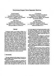
There are more than 3000 descriptors that fall into 24 groups in the PCLIENT web database, different descriptors in the same grouping have similar physicochemical properties. The 18 descriptors screened out are mapped to the molecular physiochemical property groups provided by PCLIENT shown in Table 3. These descriptors are distributed in 11 molecular physiochemical property groups. The model built on the 18 descriptors has a high precision either in terms of fitting prediction or in terms of independent prediction. Figure 1 compares the independent test set predicted value of the SVR model and the experimental value. It can be seen that most sample

284

Maximal Information Coefficient and Support Vector Regression Based Nonlinear Feature Selection and QSAR Modeling J. Braz. Chem. Soc.

points fall nearby the line of 45°. The error between the experimental value and the predicted value is small, meaning that the 18 descriptors screened out have a high significance. The SVR model has a high robustness.

Xternal Validation Plus42,43 is a tool which computes all the required external validation parameters, while further it also judges the performance of prediction quality of a QSAR model based on the MAE-based criteria. We take the 30 independent test samples as input to validate. The MAE-based metrics estimated that the model shows ‘GOOD’ predictions (after removing 5% test set objects with high residual values).

Conclusions

Figure 1. Experimental value and predicted value of the independent test set based on SVR (support vector regression) model. Take the 18 descriptors as input features and take the 30 samples (see Table 1) as independent test set, then calculating the pIGC50 values (predicted values) by SVR. The closer the circle mark is to the diagonal line, the better is the predict performance. Table 3. Physicochemical property groups of the 18 reserved descriptors Group

Descriptor

Molecular properties

ALOGP, ALOGP2

BCUT descriptors29

BEHm1, BELm4, BELm8

28

IDMT, Vindex, Xindex

Information indices30 Walk and path counts

MPC08, MPC09

3D-MoRSE descriptors32

Mor03p, Mor31e

Topological descriptors33

HyDp

Geometrical descriptors34

DDI,

31

EEig04d

Edge adjacency indices

35

Topological charge indices36

GGI5

Constitutional descriptors37

nC

Eigenvalue-based indices

38

VEe2

External validation of test set

Enalos Nodes are cheminformatics tools developed by NovaMechanics Ltd.39,40 It is a package of KNIME software, so we can use Enalos Nodes after the package are installed on KNIME.41 Enalos Nodes contains four nodes, we use the Applicability Domain (APD) based on the Euclidean distances to verify the domain of applicability. Take the data of training set (Y are excluded) and test set (Y are excluded) as input, the results showed that only one sample are unreliable in 30 samples.

PCLIENT is used to represent the alcohol organic small molecule compounds. Every compound obtains 1,388 physiochemical parameter descriptors, covering multiple properties, such as hydrophobicity, topography, electrophilicity and three-dimensional property. The properties of the alcohol organic small molecule compounds are comprehensively and systematically represented. However, in terms of the QSAR model, the irrelevant, redundant descriptors can influence the prediction precision. Thus, this paper first calculates the MIC of all descriptors. Then, based on the p-value corrected by Bonferroni, 282 descriptors whose significance value is below 0.05 are screened out. After multiple round of backward elimination, 138 critical physiochemical descriptors are retained, mRMR-MIC method is further employed to filtering the variable set, 18 descriptors are screened out in the end. Based on the 18 molecule descriptors, the SVR algorithm is employed to build the QSAR model. The newly-built QSAR model is then applied to predict the biotoxicity of test samples, and the prediction results are favorable. The prediction indexes, Q2 and RMSEP, reach 0.940 and 0.277, respectively. Compared with the classical statistical models, MLR and PLS regression, the model proposed in this paper is significantly superior, and has promising prospects to be further applied to QSAR research of toxicity of alcohol organic small molecule compounds.

Acknowledgments This work was supported by the National Natural Science Foundation of China (No. 31601652 and 31701164), the Natural Science Foundation of Hunan Province, China (No. 2016JJ6060), the National Key R&D Program of China (No. 2017YFD0301505), the Open Research Program of Hunan Provincial Key Laboratory for Germplasm Innovation and Utilization of Crop (No. 15KFXM11).

References 1. Grady, C. P.; J. Environ. Eng. 1990, 116, 805.

Vol. 30, No. 2, 2019

285

Wang et al.

2. Budi, S.; Suliasih, B. A.; Othman, M. S.; Heng, L. Y.; Surif, S.; Waste Manage. 2016, 55, 231. 3. Abraham, M. H.; Rafols, C.; J. Chem. Soc. 1995, 2, 1843. 4. Puzyn, T.; Rasulev, B.; Gajewicz, A.; Hu, X.; Dasari, T. P.; Michalkova, A.; Hwang, H. M.; Toropov, A.; Leszczynska, D.; Leszczynski, J.; Nat. Nanotechnol. 2011, 6, 175. 5. Karelson, M.; Lobanov, V. S.; Katritzky, A. R.; Chem. Rev. 1996, 96, 1027.

23. Székely, G. J.; Rizzo, M. L.; Bakirov, N. K.; Ann. Stat. 2007, 35, 2769. 24. Zhang, H.; Li, L.; Chao, L.; Sun, C.; Yuan, C.; Dai, Z.; Yuan, Z.; BioMed Res. Int. 2014, 9, 589290. 25. https://ww2.mathworks.cn/help/stats/regress.html?s_ tid=srchtitle, accessed in August 2018. 26. Vapnik, V.; Technometrics 2012, 38, 409. 27. Tropsha, A.; Gramatica, P.; Gombar, V. K.; QSAR Comb. Sci.

6. Chang, C. C.; Lin, C. J.; ACM Trans. Intell. Syst. Technol. 2011,

2003, 22, 69. 28. Galvez, J.; Garcia, R.; Salabert, M. T.; Soler, R.; J. Chem. Inf.

2, 27. 7. Xu, J.; Tang, Y. Y.; Zou, B.; Xu, Z.; Li, L.; Lu, Y.; IEEE Trans. Cybern. 2015, 45, 1169. 8. Suykens, J. A. K.; Vandewalle, J.; Neural Process. Lett. 1999,

Comput. Sci. 1994, 34, 520. 29. Burden, F. R.; J. Chem. Inf. Comput. Sci. 1989, 29, 225. 30. Balaban, A. T.; Balaban, T. S.; J. Math. Chem. 1991, 8, 383. 31. Ruecker, G.; Ruecker, C.; J. Chem. Inf. Comput. Sci. 1993, 33,

9, 293. 9. Zhou, W.; Wu, S.; Dai, Z.; Chen, Y.; Xiang, Y.; Chen, J.; Sun, C.; Zhou, Q.; Yuan, Z.; Chemom. Intell. Lab. Syst. 2015, 145,

683. 32. Schuur, J.; Selzer, P.; Gasteiger, J.; J. Chem. Inf. Comput. Sci. 1996, 36, 334.

30. 10. Norinder, U.; Neurocomputing 2003, 55, 337.

33. Diudea, M. V. J.; J. Chem. Inf. Comput. Sci. 1996, 36, 535.

11. Doucet, J. P.; Barbault, F.; Xia, H.; Barbault, F.; Doucet, J. P.;

34. Nikolic, S.; Trinajstic, N.; Mihalic, Z.; Chem. Phys. Lett. 1991,

Curr. Comput.-Aided Drug Des. 2007, 3, 263. 12. Wang, L.; Dai, Z.; Zhang, H.; Bai, L.; Yuan, Z.; Chem. Biol. Drug Des. 2014, 83, 379. 13. Li, F.; Liu, J.; Cao, L.; Emerging Contam. 2015, 1, 8. 14. Reshef, D. N.; Reshef, Y. A.; Finucane, H. K.; Science 2011,

179, 21. 35. Estrada, E.; J. Chem. Inf. Comput. Sci. 1995, 35, 31. 36. Galvez, J.; Garcia, R.; Salabert, M. T.; Soler, R. J.; J. Chem. Inf. Comput. Sci. 1994, 34, 520. 37. Todeschini, R.; Consonni, V.; Handbook of Molecular Descriptors; Wiley: Weinheim, 2000.

334, 1518. 15. Tetko, I. V.; Gasteiger, J.; Todeschini, R.; Mauri, A.; Livingstone, D.; Ertl, P.; Palyulin, V. A.; Radchenko, E. V.; Zefirov. N. S.; Makarenko, A. S.; J. Comput.-Aided Mol. Des. 2005, 19, 453. 16. Dai, Z.; Wang, L.; Chen, Y.; Wang, H.; Bai, L.; Yuan, Z.; Amino Acids 2014, 46, 1105.

38. Balaban, A. T.; Ciubotariu, D.; Medeleanu, M.; J. Chem. Inf. Comput. Sci. 1991, 31, 517. 39. https://www.knime.com/community/enalos-nodes, accessed in August 2018. 40. Melagraki, G.; Afantitis, A.; RSC Adv. 2014, 4, 50713.

17. http://www.molinspiration.com/jme/, accessed in August 2018.

41. https://www.knime.com, accessed in August 2018.

18. http://vcclab.org/lab/pclient/, accessed in August 2018.

42. http://teqip.jdvu.ac.in/QSAR_Tools/, accessed in August 2018.

19. http://www.exploredata.net/Downloads/P-Value-Tables,

43. Roy, K.; Kar, S.; Ambure, P.; Chemom. Intell. Lab. Syst. 2015,

accessed in August 2018.

145, 22.

20. https://cran.r-project.org/web/packages/minerva/index.html, accessed in August 2018. 21. Peng, H.; Long, F.; Ding, C.; IEEE Trans. Pattern Anal. Mach.

Submitted: May 25, 2018 Published online: September 11, 2018

Intell. 2005, 27, 1226. 22. Deng, X.; Tan, S.; Chen, Y.; Yuan, Z.; Res. J. Biotechnol. 2016, 11, 81.

This is an open-access article distributed under the terms of the Creative Commons Attribution License.