ISSN(Print) 1975-0102 ISSN(Online) 2093-7423
J Electr Eng Technol Vol. 8, No. 5: 991-1001, 2013 http://dx.doi.org/10.5370/JEET.2013.8.5.991
Maximization of Transmission System Loadability with Optimal FACTS Installation Strategy Ya-Chin Chang† and Rung-Fang Chang* Abstract – Instead of building new substations or transmission lines, proper installation of flexible AC transmission systems (FACTS) devices can make the transmission networks accommodate more power transfers with less expansion cost. In this paper, the problem to maximize power system loadability by optimally installing two types of FACTS devices, namely static var compensator (SVC) and thyristor controlled series compensator (TCSC), is formulated as a mixed discrete-continuous nonlinear optimization problem (MDCP). To reduce the complexity of the problem, the locations suitable for SVC and TCSC installations are first investigated with tangent vector technique and real power flow performance index (PI) sensitivity factor and, with the specified locations for SVC and TCSC installations, a set of schemes is formed. For each scheme with the specific locations for SVC and TCSC installations, the MDCP is reduced to a continuous nonlinear optimization problem and the computing efficiency can be largely improved. Finally, to cope with the technical and economic concerns simultaneously, the scheme with the biggest utilization index value is recommended. The IEEE-14 bus system and a practical power system are used to validate the proposed method. Keywords: FACTS, Network congestion, PI sensitivity factor, SVC, Static voltage Stability, Transmission system loadability, TCSC, Tangent vector technique
of the load-flow Jacobian and the controllability characteristics of an equivalent state model, were used to study the voltage instability phenomenon as well as to assess the potential for small-signal voltage stability improvement. A linear programming based optimal power flow (OPF) method was used in [5] to speed up the control to FACTS devices when contingencies happen, and thus fast decision of load shedding was made for overload and irregular voltage. While in [6], by using a mixed integer optimization technique, the demand responses and the SVC and TCSC controllers were optimally coordinated with the conventional generators to manage the network congestion under a restructured market environment. To speed up the approach to the optimal solution of the MDCP directly, a fitness sharing technique based PSO solution algorithm was proposed in [7] by diversifying the search region of the particles as much as possible. In [8], a user-friendly FACTS placement toolbox, Graphical User Interface (GUI), was developed to maximize the transmission system loadability by optimizing the locations and sizing parameters of multi-type FACTS devices, such as SVC, TCSC, TCVR, TCPST and UPFC, by using a genetic algorithm (GA). It was demonstrated to be effective and flexible enough for the users to analyze a great number of scenarios for a large power system. To lessen the computing burden to solve the discrete variables in an optimal FACTS installation problem two step approaches were adopted in [9-11]. First, the locations suitable for installations of different types of FACTS devices were investigated by analytical techniques, and then optimal
1. Introduction Under constantly increased electricity demands and power transactions, it is becoming more essential to enhance the system loadability of existing transmission networks such that more power transfers can be accommodated with less network expansion cost. Instead of mechanically switched controllers, use of FACTS devices for power-flow control is preferable as it can achieve higher levels of series compensation, different types of compensation (or a combination of them) in one device, higher reliability, as well as faster and smoother control [1]. TCSC, SVC and unified power flow controller (UPFC) can be used to balance the transmission line flows and system voltage, leading to lower system losses and higher loadability. Most of the studies on optimal FACTS installation are oriented to technical, economic or both concerns. In technical concerns, the method proposed in [2] practically installed different FACTS devices on different locations to identify the increase of loadability. While in [3], the genetic algorithm (GA) was used to select suitable locations for FACTS installation to maximize system security as well as improve loadability. With the compensation of SVC, TCSC and UPFC installations, in [4], the singular value/eigenvalue decomposition analysis †
Corresponding Author: Dept. of Electrical Engineering, Cheng Shiu University, Kaohsiung, Taiwan (
[email protected]) * Dept. of Electrical Engineering, Kao Yuan University, Kaohsiung, Taiwan. Received: February 13, 2013; Accepted: April. 29, 2013
991
Maximization of Transmission System Loadability with Optimal FACTS Installation Strategy
power flow (OPF) methods were utilized to determine the best controls to maximize system loadability. While in economic concerns, in [12] and [13], with the sum of FACTS installation and generation costs as the objective function, GA was utilized to make decision where to install the FACTS devices. The method proposed in [14] was aimed to determine the optimal locations and settings for SVC and TCSC installations by using a PSO algorithm to mitigate small signal oscillations in a multimachine power system. While the strategy proposed in [15], comprised of the tabu search (TS) and a nonlinear programming method, was utilized to optimize FACTS devices investment and recovery. With the proposed performance indices of real power flows, the method developed in [16] was used to seek the optimal FACTS devices installation locations. Under the existing FACTS devices, in [17], the minimum generation cost based OPF problem was solved by the proposed hybrid of TS and simulated annealing (SA) algorithms. While in [18], an optimal strategy comprising CPF and OPF techniques to install the static model of UPFC, was proposed by minimizing the sum of the generation cost and investment. The hybrid immune algorithms (HIA) proposed in [19], with the performance validated to be better than other evolutionary methods such as GA, PSO, and IA, were utilized to increase system loadability by optimizing the locations for UPFC installation. The new indices, thermal capacity index (TCI) and contingency capacity index (CCI), proposed in [20] were used to place TCSC at appropriate location under normal and network contingency conditions respectively. In [21], with the genetic algorithm (GA) method proposed, the FACTS devices, SVC, TCSC, TCVR and TCPST, were optimally placed by minimizing the total cost of the generation and the installed FACTS devices. To cope with both concerns simultaneously, in [22], with a single-objective function linearly composed of voltage security, system loss, capacities for STATCOM installation and loading margin (LM), the optimal STATCOM installation problem was solved by using a PSO algorithm. While in [23] and [24], a single-objective function based was linearly composed of the installation costs for various types of FACTS devices, UPFC, TCSC and SVC, system securities and loss, and voltage stability indices, and the OPF problem was solved by PSO in [23] and GA in [24]. Besides, to reveal the variety of solutions as far as possible, the optimal FACTS installation problem for LM enhancement was formulated as a multi-objective optimization problem (MOP). With the developed strategy including fuzzy logic and real coded genetic algorithm, [25] proposed a fuzzy performance index, based on distance to saddle node bifurcation, voltage profile and capacity of shunt FACTS controller, to find the most effective location and optimal size of the shunt FACTS devices, SVC or STACOM. Under the aim to release low voltage problem and line congestion, [26] applied a multiobjective genetic algorithm (MOGA) to the combinatorial
optimization problem with the multi-objective function composed of minimum FACTS installation cost and allowable system security limits. The results obtained include the FACTS devices used, the installation locations and capacities. While in [27], with the minimum generation costs and system security limits involved in the multiobjective function, a bacterial swarming algorithm (BSA) was used to determine the locations and capacities for the installations of various types of FACTS devices (TCSC, TCPST, TCVR, SVC). In [28], with the multi-objective function composed of maximum LM, minimum system loss and voltage deviations at PQ buses, an MOPSO method was applied to solve for the locations and capacities for one SVC and one TCSC installations. The method proposed in [29], with the generation cost, the investment cost for FACTS installation and the transmission security functions taken into account in a multi-objective GA algorithm, is used to determine what types of FACTS devices, where to install and their capacities. With minimum installation cost and maximum system loadability as the objective, a PSO approach was proposed in [30] to directly optimize the locations and capacities for the installations of different numbers of TCSC, SVC and/or UPFC by a step-by-step strategy. In the paper, both concerns are considered. The CPF technique [31, 32] is employed to formulate the MDCP to determine the optimal locations and capacities for TCSC and SVC installations by respecting bus voltage magnitude limits and line thermal ratings. To reduce the computing burden of the MDCP, the analytical approaches are adopted. First, the locations suitable for SVC and TCSC installations are investigated with tangent vector technique and PI sensitivity factor respectively and then, with the locations considered for SVC and TCSC installations, a set of schemes is simply formed. The MDCP for each scheme with the specific locations for SVC and TCSC installations is then reduced to a continuous nonlinear optimization problem and solved by using a guaranteed convergence particle swarm optimization (GCPSO) based OPF method [9, 33]. Finally, the scheme with the biggest utilization index value is suggested. The utilization index is defined as the ratio of the loading factor value to the investment for the SVC and TCSC installations. The modified IEEE-14 bus system and the simplified Taipower transmission network are used to validate the performance of the proposed method.
2. Problem Formulation 2.1 Effects of SVC and TCSC installations Assuming bus i to be a PQ bus and Qci a continuously regulable reactive power provided by the SVC installation at the bus, the settings are limited within: −Qc ≤ Qci ≤ Qc . The equivalent injection at bus i with an SVC installation 992
Ya-Chin Chang and Rung-Fang Chang bus-i ' where gij =
PDio + jQ Dio + λ ( ∆PDi + j∆QDi )
jQci
is shown in Fig. 1 and, with the loading factor λ used to make system demands increase, the real and reactive power balance equations are expressed as: ij , c
ij , c
+ PDio + λ∆PDi = 0
+ QDio − Qci + λ∆QDi = 0
(2)
− PGio − PGi + PDio + λ∆PDi = 0
(3)
− QGio − QGi + QDio + λ∆QDi = 0
(4)
∀j
∑Q
ij , c
∀j
Pij ,c = Vi 2 gij' − ViV j (gij' cos θ ij + bij' sin θij )
(5)
Qij , c = −Vi (b + bsh ) − ViV j (g sin θij − b cos θ ij )
(6)
' ij
' ij
rij + jxij
bus − i
' ij
− jx ij,c
jbsh
(r + xij2 )[rij2 + (xij − xij ,c ) 2 ]
,
− xij ,c (rij2 − xij2 + xij ,c xij ) (rij2 + xij2 )[rij2 + (xij − xij ,c ) 2 ]
(9)
where Dmn , h are the DC load flow sensitivity factors associating the real power flow on line m-n to the equivalent injection power Phc of a TCSC connected to bus h. s in (9) indicates the swing bus.
2.2 System loadability enhancement problem The power flow balance equations in (1) to (4) are expressed in a functional vector as follows:
g (x,v) = 0
(10)
where system variables vector x = [V θ]T including bus voltage magnitudes and phase angles, and in control variables vector v = [PG Cf F]T , PG including the real power generations, Cf including the settings of the automatic voltage regulators (AVRs), on-load tap changing (OLTC) transformers and shunt capacitors (SCs), and F including the locations and settings for the SVC and TCSC installations and loading factor λ . The operating security constraints are expressed as:
jbsh
bus − j
S jc
Sic
xij ,c rij (xij2,c − 2 xij ) 2 ij
N for line m − n ≠ line i − j ∑ Dmn, h Phc h =1 h ≠ s Pmn ≈ N D P + P for line m − n = line i − j mn , h hc jc ∑ h =1 h ≠ s
bus − j
Z ij = rij + jx ij
(8)
The real power flow on line m-n with a TCSC installation on line i-j, can be estimated by using DC power flow equations as follows [34]:
(a) bus − i
.
Pjc ≈ V ∆g ij − ViV j (∆g ij cos θ ij − ∆bij sin θ ij )
∆bij =
where Pij ,c and Qij ,c are real and reactive line flows on line i-j including the effects of the TCSC installations in the network, − PGio + PDio and −QGio + QDio are the base real and reactive injections at the bus, ∆PDi and ∆QDi are the loading level for the load at the bus to increase, and PGi and QGi are the additional real and reactive power generations for providing increased system load. As shown in Fig. 2a, letting xij ,c be the reactance provided by the TCSC installation on transmission line i-j, which is set to be regulated in compensation levels [-0.8, 0.2] and thus the settings are limited within: −0.8 xij ≤ − xij ,c ≤ 0.2 xij , where xij being the reactance of line i-j . Then, the real and reactive power flows in (1) to (4) can be expressed as:
2
r + (xij + xij ,c ) 2
(7)
Where ∆gij =
While bus i is assumed to be a PV bus, the real and reactive power balance equations are expressed as: ij , c
−(xij + xij ,c ) 2 ij
Pic ≈ Vi 2 ∆g ij − ViV j (∆g ij cos θ ij + ∆bij sin θ ij )
(1)
∀j
∑P
' and bij =
2 j
∀j
∑Q
r + (xij + xij ,c )
2
Fig. 2b shows an equivalent injection model for the branch with a TCSC installation. Equivalent real power injections at the terminal buses representing the effects of the TCSC installation on the network are [10]:
Fig. 1. A PQ bus with an SVC installation
∑P
rij 2 ij
h ≤ h(x,v) ≤ h
(11)
(b) Eq. (11) includes the limits of bus voltage, V i ≤ Vi ≤ V i ,
Fig. 2. Branch with a TCSC installation and the equivalent injection model
real and reactive generation outputs: 0 ≤ PGio + PGi ≤ PGi
993
Maximization of Transmission System Loadability with Optimal FACTS Installation Strategy
and 0 ≤ QGio + QGi ≤ QGi , line thermal ratings:
where vector ∆PG including the increments of all real power generations, for generator i, ∆PGi = PGi / λ * ; vectors ∆PD and ∆Q D including all the loading levels for system load to increase; and vectors ∆θG , ∆θ D and ∆VD being the corresponding changes of the bus angles and voltage magnitudes due to the increased system load. In general, the changes of the voltage magnitudes are negative. The factor ∆Vi / Vi is used to evaluate how necessary the SVC installation at bus i is for the system with the increased loadability able to operate within the voltage security limits. In principle, the more ∆Vi / Vi is negative, the more bus i will be necessary for an SVC installation. In the proposed strategy, since the buses with most negative ∆V / V are specified as the locations for SVC installation, the discrete variables of the MDCP to determine the locations for SVC installation can be eliminated.
Sij =
Pij2,c + Qij2,c ≤ S ij , and the capacity limits for SVC and TCSC installations. The MDCP is formulated below:
Max
λ
s.t. g (x,v) = 0 h ≤ h(x,v) ≤ h
(12)
v≤v≤v Once the problem is solved, the increased system load, λ* ∑ ∆PDi , and the optimal SVC and TCSC installations can be obtained.
3. Proposed Strategy
3.1.2 Performance index sensitivity factor
The procedure of the proposed strategy to determine a best SVC and TCSC installation scheme for suggestion is depicted in Fig. 3. The key approaches in the strategy are introduced below.
The congestion level of the transmission network can be evaluated by PI, as defined below: w PI = ∑ mn ∀mn 2k
Under the base case and without FACTS installation, use the GCPSO method to solve the loadability maximization problem
Pmn Pmn
2k
(14)
where Pmn being the real power flow on line m-n and Pmn represents the capacity; wmn being a weight to reflect the importance of the line, in the paper, which is set to 2 Pmn / Pmn and exponent k being set to 2. As a TCSC installation on line i-j, the PI sensitivity factor due to the reactance provided by the TCSC can be calculated by [10]:
Determine the locations suitable for SVC and TCSC installations using tangent vector and PI sensitivity factor respectively, and then combine the specified locations into a set of schemes For each scheme, the GCPSO method is used to maximize loadability by determining the settings for the SVC and TCSC installations Comparing the utilization indices of all schemes, the scheme with the biggest utilization index value is suggested
4
NB ∂PI 3 1 ∂Pmn = ∑ wmn Pmn ∂xij , c ℓ =1 Pmn ∂xij , c
Fig. 3. Proposed strategy
(15)
3.1 Analytical approaches where xij ,c being the reactance provided by the TCSC on line i-j. Using (9), the sensitivities of the real power flow changes associated with the change of xij ,c can be derived from:
In order to lessen the computing burden of the MDCP, the locations suitable for SVC and TCSC installations are first investigated by the respective analytical approaches.
3.1.1 Tangent vector technique Under the condidtion without FACTS installation, the MDCP in (12) becomes a continuous nonlinear optimization problem and is first solved by using the GCPSO-based OPF method [9, 33]. And then, as refer to [35, 36], with the Jacobian matrix, the changes of the state variables can be evaluated by the tangent vector as follows: ∆θG ∆PG ∆θ = J −1 ∆P D [ o] D ∆VD ∆Q D
∂P mn ∂xij ,c
∂Pjc ∂P Dmn,i ic + Dmn, j for line m − n ≠ i − j ∂xij ,c ∂xij ,c = ∂Pjc ∂Pjc ∂Pic Dmn,i ∂x + Dmn, j ∂x + ∂x for line m − n = i − j ij ,c ij ,c ij ,c (16)
As seen in (16) that if the PI sensitivity factor at line m-n is negative due to the TCSC installation on line i-j, the congestion level of line m-n can be decreased and system loadability may thus be improved. Accordingly, by
(13)
994
Ya-Chin Chang and Rung-Fang Chang
where rj is a random number sampled from U ( − 1, 1) , and ρ (k ) is a scaling factor determined by:
calculating the PI sensitivity factor in turn for each single line with a TCSC installation, it is supposed that the lines with more negative PI sensitivity factor values are more suitable for TCSC installation. Since in the proposed strategy the lines with most negative PI sensitivity factor values are specified as the locations for TCSC installation, the discrete variables of the MDCP to determine the locations for TCSC installation can also be eliminated. In the proposed strategy, the two analytical approaches are first applied to investigate the buses and lines suitable for SVC and TCSC installations and then, with the most serious K buses and most serious H lines specified for SVC and TCSC installations respectively, Κ Η Κ! Η! ⋅∑ there are ∑ schemes simply p =1 (Κ − p )!⋅ p! q =1 (Η − q )!⋅ q! formed. With the specific buses and lines for SVC and TCSC installations, the MDCP of each scheme is reduced to a continuous nonlinear OPF problem and solved using the GCPSO-based solution algorithm.
ρ (0) = 1.0, and
In traditional PSO algorithm, particle position and velocity are updated using the two equations below [37]:
vi , j (k + 1) = wvi , j (k ) + c1r1, j (pbesti , j − xi , j (k )) + c2 r2, j (gbest j − xi , j (k ))
(17)
1) Set the GCPSO iteration number and particle number in the swarm. 2) Narrow down the control variable adjustment ranges and generate a swarm. 3) A load flow computation is conducted for each particle i with X i = [PGi QCi XiL λ ]T . If no load flow solution exists in the 30 particles, return to step 2. Otherwise, set pbest and fitness for each particle. For the particles with a converged load flow solution, fitness = λ /(1 + pene _ v) , and for the particles without a load flow solution, fitness = −10 , where pene_v is a penalty proportional to the severity of security constraint violation and λ is the current loading factor. Set Ite_num=0 and go to step 4. 4) Ite_num = Ite_num+1, gbest = the pbest of the particle with maximum fitness. Restore the control variable adjustment range to the original problem and update the particles using (17)-(20). 5) Execute load flow program for each particle and check security constraints. Update particle fitness ( fitness = λ /(1 + pene _ v) ). If Ite_num is lower than the iteration number set, go to step 4, otherwise, go to step 6. 6) Record the SVC and TCSC control settings, generation outputs and loading factor value.
(18)
X i (k ) and Vi (k ) represent the position and velocity of particle i at iteration k. xi , j is the jth entry of X i (k ) . In the paper, with the assumption that the settings of all control devices (AVR, OLTC, SC) are fixed as in the base case, X i = [PGi QCi XiL λ ]T where the control variables vectors PGi including all generations, QCi including all reactive power settings for the SVC installations, XiL including all reactance settings for the TCSC installations, and λ being the loading factor. vi , j is the jth entry of Vi that denotes the velocity of X i (k ) , 0 ≤ w ≤ 1 is an inertia weight determining how much the particle’s previous velocity is preserved, c1 and c2 are two positive acceleration constants, r1, j , r2, j are random numbers sampled from uniform distribution U (0, 1) , and pbesti and gbest are the personal best position of particle i and the best position in the entire swarm, respectively. In early stages of the PSO procedure, the phenomenon of stagnation addressed in [33] may occur and could lead to a prematurely converged solution. To improve the efficiency of achieving the optimal solution, in the proposed GCPSO-based solution method, the velocity update for the best particle is modified by the following equation: vi , j (k + 1) = wvi , j (k ) − xi , j (k ) + pbesti , j + ρ (k )rj
(20)
where sc and f c are tunable threshold parameters. In this study, they are set to 15 and 10 respectively. In each iteration of the GCPSO algorithm, if there is an overall improvement of fitness that is due to the same particle as in the previous iteration, the #success index is increased and #failure is set to 0. If there is no fitness improvement for k iterations, then #failure=k, and #success is set to 0. The scaling factor of the particle velocity in (19) is updated according to Eq. (20) when #success or #failure is greater than a specified number. On the other hand, if the improvement of fitness is obtained from different particles, both #success and #failure are set to 0, and the scaling factor remains the same. For each scheme, the GCPSO-based solution algorithm proposed to maximize system loadability by determining the settings of the SVC and TCSC installations is shown below:
3.2 Solution algorithm
X i (k + 1) = X i (k ) + Vi (k + 1)
if # success > sc 2 ρ (k ) ρ (k + 1) = 0.5 ρ(k ) if # failure > f c ρ(k ) otherwise
The costs (KUSD$), f S and fT , for the SVC and TCSC installations of each scheme are calculated as [30]:
(19)
995
Maximization of Transmission System Loadability with Optimal FACTS Installation Strategy
f S = ∑ (0.0003Qci2 − 0.3051Qci + 127.38) ⋅ Qci
(21)
fT = ∑ (0.0015Qtl2 − 0.7130Qtl + 153.75) ⋅ Qtl
(22)
∀i
∀l
scheme 5, as will be detailed later, it can be found from Tables 1 and 2 that, since the voltage magnitudes at all PQ buses are within the security limits and four lines utilized up to the thermal ratings, system loadability is thus improved in a large amount. Obtained from tangent vector technique and PI sensitivity factor respectively, the three most negative
2 where Qci and Qtl = I l xl ,c being the e reactive power capacities (Mvar) for the SVC and TCSC installations on bus i and line l [1] respectively. The investment cost for the SVC and TCSC installations of each scheme is f S + fT . Eventually, one of the two utilization indices defined below are used to determine a best scheme for suggestion:
U = Loadability /(Investment cost)
(23)
U = Loadability /(Number of FACTS units)
(24)
Table 1. Load flows at base-case and when operating on system loadabilities without and with FACTS installation
4. Test Results and Discussions 4.1 Modified IEEE-14 bus system The modified IEEE-14 bus network shown in Fig. 4 is used to examine the performance of the proposed method. The base-case load flow is shown in Table 1 and the loading level is set to the base load. Taking bus voltage magnitudes within 0.9 p.u. and 1.1 p.u. and line thermal ratings as the security constraints, under without FACTS installation and when system operating at the system loadability, the load flow and line flows are shown in Tables 1 and 2, respectively. As seen in Table 1 that from the injection of bus 14, the loading factor value is calculated as λ * = (0.2372 − 0.149) / 0.149 = 0.593 . Since the voltage magnitude at bus 14 is 0.90 p.u., in order to improve system loadability, reactive power compensation close to bus 14 will be necessary. Also, as found from Table 2 that only line 7-9 is utilized sufficiently, in order for the network to accommodate more power transfers, power flow regulation is thus necessary. With the SVC and TCSC installations of
Table 2. Line flows operating on system loadabilities without and with FACTS installation
13 14 12 11 10
G
1 6
8
9
C
7
5
Table 3. Increased loading factor values resulted from the SVC and TCSC installations of various schemes
4
2 G
3
G : Generator C : Synchronous Compensator G
Fig. 4. IEEE-14 bus test system 996
Ya-Chin Chang and Rung-Fang Chang
Table 4. Investment costs (MUSD$) for the SVC and TCSC installations of various schemes
1
base case scheme 5 scheme 49
V o lta g e m a g n itu d e (p u .) o n b u s 1 4
0.9
0.8
0.7
0.6
0.5
0.4
0.3
0.2
0.1
voltage change ratios ( ∆Vi / Vi ) are found to be -0.208, 0.188 and -0.180 at buses 14, 13, and 12 respectively with an SVC installation, and the three most negative PI sensitivities are found to be -4.62, -3.78 and -1.03 on lines 1-5, 5-6 and 4-9 respectively with a TCSC installation. Formed with the three buses and three lines specified for SVC and TCSC installations, the number of the schemes is 3 3 3! 3! ⋅∑ = 49 . The loading factor ∑ p =1 (3 − p )!⋅ p! q =1 (3 − q )! ⋅ q ! values increased and the investment costs for the SVC and TCSC installations of all schemes computed from the proposed GCPSO-based solution method are shown in Tables 3 and 4 respectively. The schemes are numbered with the superscripts on the increased loading factor values and the investment costs. For example, scheme 5 contains bus 12 and lines 1-5 and 5-6 and scheme 32 contains buses 12 and 14 and lines 1-5 and 4-9, for SVC and TCSC installations respectively. It can be found from Tables 3 and 4 that in the shadow areas, the seven schemes can derive larger loadabilities with less investment costs. Using (23), the utilization index value resulted from the SVC and TCSC installations of 2 scheme 5 can be calculated as 0.0987 ⋅ ∑ ∆PDi ⋅10 / 4.71 =
0
0
0.5
1
1.5
2
2.5
Loading Margin (Lambda)
Fig. 6. P-V curves for the three study cases 2.998 MW/MUSD , which is the biggest of all schemes. The settings for the SVC and TCSC installations of scheme 5 are shown in Table 5 and the corresponding load flow and line flows can also be found in Tables 1 and 2, respectively. As can be seen in Table 1 that the voltage magnitudes at bus 14 are increased from 0.90 p.u. to 0.915 p.u., and in the shadow areas of Table 2 that lines 1-5, 2-4, 2-5 and 3-4 are all utilized up to their thermal ratings, revealing the installations can enable the network to accommodate more power transfers by sufficiently using the transfer capacity. Thus, the SVC and TCSC installations of scheme 5 are suggested for the network reinforcement. The profiles of the PQ bus voltage magnitudes derived from maximizing the system loadability of the three study cases: 1) without FACTS installation, 2) with the SVC and TCSC installations of scheme 5, and 3) with the SVC and TCSC installations of scheme 49, are shown in Fig. 5. Obviously, the system security can be effectively improved by the respective SVC and TCSC installations of the two schemes. And, obtained with the CPF method [30], the respective P-V curves of the three study cases are shown in Fig. 6. As seen that the static voltage stability can also be largely improved by both schemes. Due to the fact that scheme 5 is the most cost-effective of all schemes it is further identified to be the best suggestion.
∀i
Table 5. Locations and settings for the SVC and TCSC installations of scheme 5
*The units for SVC and TCSC are 100MVar and line compensation
4.2 Taiwan power system
level.
The simplified Taipower 345kV transmission network with 76 buses, including 50 PQ buses and 25 PV buses, and 113 transmission lines is also used for testing. The network is divided into three areas: north, central and south areas. One line diagram of the central part of the studied EHV system is shown in Fig. 7. The system demand and supply during peak-load hours are shown in Table 6. Demand in the north area is higher than those in the central and south areas. For most of the time, the north has to count on the support from the south. Table 6 also shows the loading factor value, λ * = 0.0206 , under the most serious
Fig. 5. Bus voltage profiles for the three study cases 997
Maximization of Transmission System Loadability with Optimal FACTS Installation Strategy 0.07
57 56 G
G 49
73 67
76
0.065
73 67
54
X: 765 Y: 0.0652
0.06
71
0.055
Lambda
72 30 31 27 G
0.05 0.045 0.04 0.035
G
33
G
23
24
25
G
26
G
32
0.03 0.025
37 38
34
39
35
0.02
40
36
44 G
28 29 43
G
0
100
200
300
400
500
600
700
800
900
1000
Solution Samples
42 41
X: 493 Y: 0.06869
X: 48 Y: 0.06652
Fig. 8. Distribution of 1000 solutions directly solved from the MDCP under the most serious N-2 contingency scenario
G
6
Table 7. The best solution directly solved from the MDCP under the most serious N-2 contingency scenario
9 11
12
18 G
13
2 19 14
G
3
14 G
1
G
4
G 5
Fig. 7. Central part of Taipower network Table 8. Respective most critical locations considered for SVC and TCSC installations
Table 6. Supply and demand at different areas, studied contingency and computed loading factor
shown in Table 7 are all in central-north areas. As can also be found that bus 31 and lines 12-32 and 32-71 appear in the two tables, conceivably they might be the most suitable for SVC and TCSC installations, respectively. For each scheme, the problem to maximize system loadability by determining the settings for the specific SVC and TCSC installations is solved by using the GCPSObased OPF solution algorithm. In the test, the utilization index defined in (24) is applied to measure the performance of the SVC and TCSC installations of each scheme. The utilization index values resulted from the SVC and TCSC installations of schemes S1, S2, S3 and S4 are shown in Fig. 9, and the installation results of the four schemes are shown in Table 9. Please note that the respective SVC and TCSC installations of the four schemes can enable the network to provide a biggest loadability among those of the schemes with a same number of FACTS devices (1 to 4 units) installations. As can be found in Fig. 9 that, although the system loadabilities resulted from the respective SVC and TCSC installations of schemes S1 to S4 are increased, the utilization index values decrease. Therefore, if a system loadability at λ* ≥ 0.060 is required, scheme S2 will be the best for suggestion. And, regarding the operations of the respective SVC and TCSC installations of the four schemes shown in Table 9, it can
*MVA base = 100MVA
N-2 contingency scenario before reinforcement. Using the GCPSO solution algorithm with 30 particles and 300 iterations, 1000 loading factors directly computed from the MDCP to determine three SVC and three TCSC installations are shown in Fig. 8. As seen that there are only three solutions with system loadabilities at λ* ≥ 0.0650 . The solution with the biggest system loadability at λ* = 0.0687 including the TCSC on lines 12-32, 32-71 and 36-42 and SVC installations at buses 18, 31 and 34, are shown in Table 7. Applying the analytical approaches, as shown in Table 8, it is found that the four most buses are 31, 32, 36 and 48 and the four most serious lines are 12-32, 14-18, 15-17 and 32-71. They are specified for SVC and TCSC installations 4 4 4! 4! ⋅∑ = 225 schemes can be and ∑ p =1 (4 − p )! ⋅ p! q =1 (4 − q )!⋅ q! formed. It can be found in Table 8 that locations of the buses considered for SVC installation similar with those
998
Ya-Chin Chang and Rung-Fang Chang 0.9 0.895
Voltage Magnitude (pu) on bus 40
System Loadability vs. Utilization Index
0.07
0.06
0.05
System loadability Utilization index
0.04
0.03
0.02
none SVC SVC on buses 36 and 48 SVC on buses 31 and 36
0.89 0.885 0.88 0.875 0.87 0.865
X: 0.8232 Y: 0.8627
0.86 0.855
0.01 S1
0.85
S2
S3
S4
0.76
0.78
0.8
0.82
X: 0.8514 Y: 0.861
0.84
0.86
Loading Margin (Lambda)
Scheme
Fig. 9. System loadabilities vs. corresponding utilization indices for the four schemes
Fig. 10. P-V curves for the three study cases Table 10. The results for the best SVC and TCSC installations obtained with the proposed strategy
Table 9. Results for the SVC and TCSC installations of the four schemes
can be formed, each with three buses and three lines for SVC and TCSC installations respectively and thus requiring about (478*16)/60/60=2.12 hours to compute on the same computer. As the results shown in Table 10, the scheme with three SVC installations on buses 31, 32 and 36 and three TCSC installations on lines 12-32, 14-18 and 32-71 can make the power system provide a loadability at λ* = 0.0692 which is bigger than that shown in Table 7, therefore validating the performance of the proposed strategy.
be found that each TCSC installation is operating up near to compensation level -0.8 and the reactive power provided by each SVC installation is bigger than 1.0 p.u.. Obviously each of the SVC and TCSC installations is playing an important role in making the network able to accommodate more power transfers. To analyze the effect of SVC installations on static voltage stability, the CPF method is applied to three study cases. In case 1, with two TCSC installations on lines 1232 and 32-71 already in each case, there is no SVC installation, in case 2 there are also two SVC installations at buses 36 and 48, and in case 3 there are also two SVC installations at buses 31 and 36. The P-V curves resulted from the three study cases are shown in Fig. 10. As seen that case 3 outperforms the others. Since the SVC and TCSC installations of scheme S4 are the same as those in study case 3, if also taking static voltage stability into consideration, scheme S4 will be a better choice. From the author’s experience, the GCPSO method takes about 478 seconds to obtain a solution by directly solving the MDCP to determine three SVC and three TCSC installations. As seen in Fig. 8, to derive the three solutions with system loadabilities at λ* ≥ 0.0650 requires about 478*1000/3/60/60=44.26 hours on an Intel Core Duo CPUE7650 2.66 GHZ and 2G RAM PC. While using the proposed strategy, with the four buses and four lines as 4! 4! ⋅ = 16 schemes shown in Table 8, (4 − 3)!⋅ 3! (4 − 3)!⋅ 3!
5. Conclusion It is expectable that the future economic developments will result in large electric demands regionally and, in the deregulated power systems, due to open access to the transmission networks a great numbers of various power transactions will incur huge changing power flows. In this view, serious threats to power system security might occur. With the analytical approaches used to investigate the locations suitable for SVC and TCSC installations, in this paper, an efficient SVC and TCSC installation strategy is proposed to enhance the system loadability such that the existing transmission networks can accommodate more power transfers with less network expansion cost. The efficiency of the proposed method is validated with the test results of the SVC and TCSC installation scheme suggested for transmission system loadability enhancement properly consistent with specific technical and economic concerns.
999
Maximization of Transmission System Loadability with Optimal FACTS Installation Strategy
Acknowledgements [14]
This study was sponsored by National Science Council under project number NSC 101-2221-E-230-025.
References [1]
[2]
[3]
[4]
[5]
[6]
[7]
[8]
[9]
[10]
[11]
[12]
[13]
[15]
T. Orfanogianni, R. Bacher, “Steady-State optimization in power systems with series FACTS devices,” IEEE Trans. Power Syst., Vol. 18, No. 1, 2003, pp. 19-26. A. A. Athamneh, W. J. Lee, “Benefits of FACTS devices for power exchange among Jordanian Interconnection with other Countries,” IEEE/PES General Meeting, June 2006. S. Gerbex, R. Cherkaoui, A. J. Germond, “Optimal location of multi-type FACTS devices in a power system by means of genetic algorithms,” IEEE Trans. Power Syst., Vol. 16, No. 3, 2001, pp. 537-544. A. R. Messina, M. A. Pe`rez, E. Herna`ndez, “Coordinated application of FACTS devices to enhance steady-state voltage stability,” Int. J Electr. Power Energy Syst., Vol. 19, No. 2, 2003, pp. 259-267. W. Shao, V. Vijay, “LP-based OPF for corrective FACTS control to relieve overloads and voltage violations,” IEEE Trans. Power Syst., Vol. 21, No. 4, 2006, pp. 1832-1839. A. Yousefi, et al., “Congestion management using demand response and FACTS devices,” Int. J Electr. Power Energy Syst., Vol. 37, No.1, 2012, pp. 78-85. Y. C. Chang, “Fitness sharing particle swarm optimization approach to FACTS installation for transmission system loadability enhancement,” J Electr. Eng. Technol., Vol. 8, No. 1, 2013, pp. 31-39.
[21]
E. Ghahremani, I. Kamwa, “Optimal placement of multiple-type FACTS devices to maximize power system loadability using a generic graphical user interface,” IEEE Trans. Power Syst., Early version, 2012.
[22]
[16]
[17]
[18]
[19]
[20]
K. Y. Lee, M. Farsangi, H. Nezamabadi-pour, “Hybrid of analytical and heuristic techniques for FACTS devices in transmission systems,” IEEE/PES General Meeting, June 2007, pp. 1-8. S. N. Singh, A. K. David, “Optimal location of FACTS devices for congestion management,” Electric Power Systems Research, 2001, pp. 71-79. S. H. Song, J. U. Limb, Seung-Il Moon, “Installation and operation of FACTS devices for enhancing steady-state security,” Electric Power Systems Research, 2004, pp. 7-15. L. J. Cai, I. Erlich, G. Stamtsis, “Optimal choice and allocation of FACTS devices in deregulated electricity market using genetic algorithms,” IEEE PES Power Systems Conference and Exposition, pp. 201207. T. S. Chung, Y. Z. Li, “A hybrid GA approach for
[23]
[24]
[25]
[26]
1000
OPF with consideration of FACTS devices,” IEEE Power Engineering Review, Feb. 2001, pp. 47-50. D. Mondal, A. Chakrabarti, A. Sengupta, “Optimal placement and parameter setting of SVC and TCSC using PSO to mitigate small signal stability problem,” Int. J Electr. Power Energy Syst., Vol. 42, No. 1, 2012, pp. 334-340. Y. Matsuo, A. Yokoyama, “Optimization of installation of FACTS devices in power system planning by both tabu search and nonlinear programming methods,” Proc. 1999 Intelligent System Application to Power System Conference, pp. 250-254. S. N. Singh, A. K. David, “A new approach for placement of FACTS devices in open power markets,” IEEE Power Engineering Review, Vol. 21, No. 9, 2001, pp. 58-60. P. Bhasaputra, W. Ongsakul, “Optimal power flow with multi-type of FACTS devices by hybrid TS/SA approach,” IEEE Proc. International Conference on Industrial Technology, Vol. 1, 2002, pp. 285-290. H. A. Abdelsalam, et. al., “Optimal location of the unified power flow controller in electrical power system,” IEEE Proc. Large Engineering Systems Conference on Power Engineering, July 2004, pp. 41-46. S. A. Taher, M. K. Amooshahi, “New approach for optimal UPFC placement using hybrid immune algorithm in electric power systems,” Int. J Electr. Power Energy Syst., Vol. 43, No. 1, 2012, pp. 899909. S. K. Sundar, H. M. Ravikumar, “Selection of TCSC location for secured optimal power flow under normal and network contingencies,” Int. J Electr. Power Energy Syst., Vol. 34, No. 1, 2012, pp. 29-37. A. A. Alabduljabbara, J. V. Milanovi`c, “Assessment of techno-economic contribution of FACTS devices to power system operation,” Electric Power Systems Research, 2010, 1247-1255. E. N. Azadani, et. al., “Optimal placement of multiple STATCOM,” The 12th International Middle-East Power System Conference, March 2008, pp.523-528. D. Povh, “Modeling of FACTS in power system studies,” IEEE/PES Winter Meeting, Vol. 2, Jan. 2000, pp. 1435-1439. H. R. Baghaee, M. Annati, B. Vahidi, “Improvement of voltage stability and reduce power system losses by optimal GA-based allocation of multi-type FACTS devices,” Int. Conf. Optimization of Electrical and Electronic Equipment, May 2008, pp. 209-214. A. R. Phadke, M. Fozdar, K. R. Niazi, “A new multiobjective fuzzy-GA formulation for optimal placement and sizing of shunt FACTS controller,” Int. J Electr. Power Energy Syst., Vol. 40, No. 1, 2012, pp. 46-53. A. S. Yome, N. Mithulananthan, K. Y. Lee, “Static voltage stability margin enhancement using STATCOM,
Ya-Chin Chang and Rung-Fang Chang
[27]
[28]
[29]
[30]
[31]
[32]
[33]
[34] [35]
[36]
[37]
TCSC and SSSC,” 2005 IEEE/PES Transmission and Distribution Conference & Exhibition, pp. 1-6. Z. Lu, M. S. Li, L. Jiang, “Optimal allocation of FACTS devices with multiple objectives achieved by bacterial swarming algorithm,” IEEE/PES General Meeting, Conversion and Delivery of Electrical Energy in the 21st Century, July 2008, pp. 1-7. A. Lai′fa, M. Boudour, “FACTS allocation for power systems voltage stability enhancement using MOPSO,” Int. Multi-Conference on Systems, Signals and Devices, IEEE SSD 2008, July 2008, pp. 1-6. D. Radu, Y. Besanger, “A multi-objective genetic algorithm approach to optimal allocation of multitype FACTS devices for power systems security,” IEEE/PES General Meeting, June 2006. M. Saravanan, et. al., “Application of particle swarm optimization technique for optimal location of FACTS devices considering cost of installation and system loadability,” Electric Power Systems Research, 2007, pp. 276-283. V. Ajjarapu, C. Christy, “The continuation power flow: a tool for steady state voltages stability analysis,” IEEE Trans. Power Syst., Vol. 7, No. 1, 1992, pp. 416423. H. D. Chiang, et. al., “CPFLOW: a practical tool for tracing power system steady-state stationary behavior due to load and generation variations,” IEEE Trans. Power Syst., Vol. 10, No. 2, 1995, pp. 623-628. F. V. D. Bergh, A. P. Engelbrecht, “A new locally convergent particle swarm optimizer,” Proc. of IEEE Conference on Systems, Man and Cybernetics (Hammamet. Tunisia), Vol. 3, 2003. A. J. Wood, B. F. Wollenberg, “Power Generation, Operation and Control,” John Wiley, New York, 1996. A. A. A. Esmin, G. L. Torres, A. C. Z. Souza, “A hybrid particle swarm optimization applied to loss power minimization,” IEEE Trans. Power Syst., Vol. 20, No. 2, 2005, pp. 859-866. A. C. Z. de Souza, C. A. Cañizares, V. H. Quintana, “New techniques to speed up voltage collapse computations using tangent vectors,” IEEE Trans. Power Syst., Vol. 12, No. 3, 1997, pp. 1380-1387. J. Kennedy, R. Eberhart, “Particle swarm optimization,” Proc. of 1995 IEEE Int. Conf. on Neural Networks (ICNN’95), Vol. IV, pp. 1942-1948.
1001
Ya-Chin Chang received Ph.D. degree from National Sun Yat-Sen University, Taiwan, in 2002. He is an associate professor with the Department of Electrical Engineering, Cheng Shiu University, Taiwan. His research interests are on power system operation and planning, and integration of distributed energy resources in distribution systems. Rung-Fang Chang received Ph.D. degree from National Sun Yat-Sen University, Kaohsiung, Taiwan, in 2002. He is an associate professor with the Department of Electrical Engineering, Kao Yuan University, Taiwan. His research interests are on optimization of power system and load management.