Maximum Entropy Deconvolution of Infrared Spectra: Use of a Novel Entropy Expression Without Sign Restriction ´ RENZ-FONFRI´A* and ESTEVE PADRO ´S VI´CTOR A. LO Unitat de Biofı´sica. Departament de Bioquı´mica i de Biologia Molecular, Facultat de Medicina, Universitat Auto`noma de Barcelona, 08193 Bellaterra, Barcelona, Spain
Absorbance and difference infrared spectra are often acquired aiming to characterize protein structure and structural changes of proteins upon ligand binding, as well as for many other chemical and biochemical studies. Their analysis requires as a first step the identification of the component bands (number, position, and area) and as a second step their assignment. The first step of the analysis is challenged by the habitually strong band overlap in infrared spectra. Therefore, it is useful to make use of a mathematical method able to narrow the component bands to the extent to eliminate, or at least reduce, the band overlap. Additionally, to be of general applicability this method should permit negative values for the solution. We present a maximum entropy deconvolution approach for the band-narrowing of absorbance and difference spectra showing the required characteristics, which uses the generalized negative Burg-entropy (Itakura–Saı¨to discrepancy) generalized for difference spectra. We present results on synthetic noisy absorbance and difference spectra, as well as on experimental infrared spectra from the membrane protein bacteriorhodopsin. Index Headings: Infrared spectroscopy; Resolution enhancement; Band narrowing; Spectral quantification; Data processing.
INTRODUCTION The interpretation of infrared spectra requires both band assignment and band quantification. The band assignment, which is a difficult and ambiguous process by itself, is severely challenged by band overlap, which precludes the correct determination of the number of bands and the direct estimation of their positions and areas. The mathematical narrowing of a spectrum would eliminate, or at least reduce, the band overlap and therefore allow a direct estimation of the number of component bands present, their position and, in most favorable cases, even their area. Consequently, the mathematical narrowing of spectra has interested the scientific community for a long time. In some cases, the widths of the bands in a spectrum are controlled by the instrumental broadening. Therefore, bands can be narrowed with the use of more resolving instrumentation, as well as mathematically. On other occasions, the widths of the bands are intrinsic to the studied system, and thus mathematical narrowing is the only alternative for obtaining more resolved spectra, i.e., with less overlap between the component bands. The narrowing of spectra has been attempted from diverse points of view, and several methods have emerged over time, namely, derivatives,1,2 inversion of the comReceived 4 May 2004; accepted 15 November 2004. * Author to whom correspondence should be sent. Present address: Department of Materials Science and Engineering, Nagoya Institute of Technology, Showa-ku, Nagoya 466-8555, Japan. E-mail: victor.
[email protected].
474
Volume 59, Number 4, 2005
plex Laplace transform,3 linear prediction by autoregressive modeling,4–6 wavelet-transform,7,8 and deconvolution. Deconvolution has become one of the most used methods for narrowing purposes. Deconvolution is an unstable process and different strategies for the stabilization of the deconvoluted solution have been proposed, namely, the use of a smoothing filter in Fourier deconvolution;1,9–12 the combination of deconvolution and linear prediction;13–16 the combination of Fourier deconvolution and wavelet transform;17,18 iterative deconvolution with constraints, also known as maximum likelihood restoration;19–21 and the application of inversion theory, in which we include related methods like regularization19,22 and probabilistic (Bayesian) methods. 23 Regularized and probabilistic methods consider the deconvolution of data as an inverse problem without a welldefined solution. These methods provide the simplest, least informative, or more probable solution among all plausible solutions. The simplicity, lack of information, or probability of a solution is often measured by a function that receives the name of entropy; hence, the name of maximum entropy is related both to regularization and probabilistic methods. Maximum entropy deconvolution seems to offer narrower spectra than Fourier deconvolution, and with less noise content. 22,24,25 On the other hand, it appears more robust than linear prediction methods, which can give rise to false peaks and artifactual band splitting. 26–28 Therefore, it can be considered as one of the more powerful and reliable band-narrowing methods in use today. However, maximum entropy deconvolution often assumes that deconvoluted data is positive everywhere, i.e., the entropy expression is not defined for negative values of the solution. Although this assumption is reasonable in astronomical image restoration, the field in which these methods were first applied, 29–31 it is not always acceptable in spectroscopy. Positive and negative values may be expected in deconvoluted spectra for mathematical reasons, for instance when (1) there exists a baseline drift; (2) spectra are not correctly phased; and (3) the band shape used in deconvolution does not match the actual band shapes in the spectrum (e.g., bands with some Gaussian character deconvoluted with pure Lorentzian bands). On the other hand, maximum entropy deconvolution algorithms restricted to positive values can fail to converge if any band is being over-deconvoluted. This problem can be solved by avoiding over-deconvolution, but often at the intolerable cost of insufficient narrowing of broader bands, as we will show. A maximum entropy deconvolution allow-
0003-7028 / 05 / 5904-0474$2.00 / 0 q 2005 Society for Applied Spectroscopy
APPLIED SPECTROSCOPY
ing for negative values can allow for slight over-deconvolution, and so be of practical utility when bands of different widths coexist in the data. These situations are likely to occur in the deconvolution of the amide I of proteins. The amide I band of proteins contains information about protein structure.32–36 The amide I band position is correlated with the protein secondary structure, as demonstrated from both experimental studies and theoretical studies on peptides with known and pure secondary structure,37–40 and from experimental studies on proteins with known structure.32,41–50 In proteins, due to the high structural heterogeneity, the amide I region becomes band crowded. In order to resolve the contributions of the different bands, a bandnarrowing mathematical method is often applied.32,46 Here resides the interest in a powerful band-narrowing method, such as maximum entropy deconvolution, which would allow the identification of more protein structures in the amide I. However, due to the high number of bands and their overlap it is hard to estimate a priori the shape and width of the amide I bands. Moreover, a non-common band shape or bandwidth for the amide I bands is conceivable. Therefore, for the deconvolution of the amide I, the use of a maximum entropy deconvolution allowing for negative values in the solution is recommended. Other times, positive and negatives values should be expected in a deconvoluted spectra for physical reasons, as for infrared lineal dichroism spectra51–53 or for difference spectra. For instance, several papers have reported infrared difference spectra corresponding mainly to protein conformational changes upon substrate binding.54–60 In the same way, temperature, pH, and urea concentration changes have been used to obtain difference spectra corresponding to protein structural changes upon folding or unfolding.61–66 Other examples are protein structural changes (or amino acid protonation changes) induced by light,67–69 by redox reactions,70,71 etc.; or spectroscopic changes induced by H/D exchange,72,73 etc. However, the identification and quantification of bands in these difference spectra is difficult due to their habitual moderate/ low signal-to-noise ratio, band overlap, and partial band cancellation between close positive and negative bands. Shannon-related entropies for positive solutions have been used frequently for the deconvolution of NMR and astronomic data.5,26,29,31,74–76 Additionally, they have been used with success in the inversion of the Laplace transform in kinetic data obtained by fluorescence, infrared, or UV-vis spectroscopy.73,77–82 In their form for solutions without a sign restriction, described more than a decade ago,83,84 they have been used frequently in nuclear magnetic resonance (NMR) spectroscopy, although rarely for deconvolution purposes. 28,83–86 In this paper, we first tested the suitability of Shannon-related entropies for the infrared deconvolution problem. Although the well-known expression for positive-restricted solutions worked very well, the form without sign restriction showed moderate band narrowing with excessive noise enhancement. Finally, we also considered entropy expressions alternative to the Shannon-related entropies, such as Burgrelated entropies, which in their original form are also restricted to positive values. We derived and used, for the first time to our knowledge, a Burg-related entropy for solutions without sign restriction. In this paper, we dem-
onstrate the suitability of this entropy expression for the infrared deconvolution problem. It shows both a high band-narrowing capability and a high insensitivity to the noise present in the data. We tested and compared the performance of both entropy expressions (Shannon-related and Burg-related) with Fourier deconvolution and with maximum likelihood restoration for the deconvolution of synthetic noisy absorption and difference spectra. Deconvolution was also tested on infrared experimental data from bacteriorhodopsin. THEORETICAL BACKGROUND Deconvolution. Narrowing by deconvolution is based on considering the measured data, g(v), the result of a blurring process plus added noise acquired at a certain instrumental resolution. A more resolved noise free data, ˆf (v) (focused data), is convolved by an intrinsic lineshape function, p(v), corrupted by noise, n(v), and convolved with the instrumental function, r(v): g(v) 5 [ ˆf (v) J p(v) 1 n(v)] J r (v) 5 fˆ (v) J h(v) 1 n(v) J r (v) 5 gˆ (v) 1 n(v) J r (v)
(1)
where gˆ(v) stands for the noise-free blurred data, J represents convolution, and h(v) is the point spread function (PSF), which collects the intrinsic line-shape function and the instrumental broadening. The focused data could be obtained by deconvolution of the noise-free data, as: fˆ (v) 5 I
5
6
[ ]
ˆ I21 [gˆ (v)] G(t) 5I 21 I [h(v)] H(t)
(2)
where I and I21 stands for the direct and inverse Fourier transform and x(v) ⇔ X(t) are Fourier pairs. In practice, since the experimental data contains noise, its deconvolution will give f (v) 5 I
[ ] [ ] [ ] [ ] ˆ G(t) G(t) N(t)R(t) 5I 1I H(t) H(t) H(t)
5 fˆ (v) 1 I
N(t)R(t) H(t)
(3)
Therefore, the deconvoluted data, f (v), is equal to the focused data plus deconvoluted noise. The inverse Fourier transform of the PSF becomes zero, or tends to, as t increases. Therefore, the solution obtained by Eqs. 2 and 3 is either indeterminable or dominated by deconvoluted noise. Some strategies have been described to solve both limitations. In order to control the noise, in Fourier deconvolution G(t) is multiplied by a filter function that attenuates/eliminates the high frequency components in g(v), resulting in a smoothed deconvoluted data.1,10,11 In wavelet Fourier deconvolution the deconvoluted data is smoothed by limiting the allowed basis functions, which represent g(v).17,18 In Fourier deconvolution combined with linear prediction, G(t)/H(t) is cut at an appropriate value of t. Then the following values are predicted from the previous ones using an appropriate autoregressive filter.13,14,27 This approach can solve the inAPPLIED SPECTROSCOPY
475
determination in Eqs. 2 and 3 when H(t) and R(t) become zero. In practice, the autoregressive filter is obtained as that accurately predicting known data. However, when the data is noisy, this approach generates an incorrect autoregressive filter, giving rise to all the known problems related to linear prediction (splitting, false peaks, etc.). 26–28 In these three methods, the presence of noise in the data is not considered in the core of the problem. A completely different approach is developed from probabilistic and regularization methods. Probabilistic Deconvolution. Deconvolution can be considered an inference problem. We aim to infer the non-blurred noise-free data, f (v), given the experimental data g(v), and the blurring function h(v). Substituting functions by vectors and applying Bayes theorem:31 Pr(f z g,h) 5
Pr(f) 3 Pr(g z f,h) Pr(g)
(4)
where Pr stands for probability, ‘‘z’’ means ‘‘given’’ and ‘‘,’’ means ‘‘and’’. Therefore, Pr(f z g,h) is the probability of f given g and h (the inference probability or posterior probability); Pr(f) is the probability of f, i.e., the probability of a solution before measurement (the prior probability); Pr(g z f,h) is the probability of g given f and h (the likelihood probability); and Pr(g) is the probability of g (the evidence probability), which can be determined by normalization. The most probable solution f is that maximizing Eq. 4, which requires the evaluation of both Pr(f) and Pr(g z f,h). Expressions for Pr(g z f,h) are well known for different types of noise present in the data. For instance, for uncorrelated Gaussian noise with constant variance: Pr(g z f,h) } Pexp(2di2 ) where d 5 g 2 fJh. On the other hand, the expression for Pr(f) has been controversial. The most accepted expression is Pr(f) } exp(a 3 S), where a is an unknown constant (that can be estimated) and S is the Shannon-related entropy of the solution.31 When the solution is a probability distribution, we should use the Shannon entropy: S 5 2 S f iln f i.87 When the solution is a positive and additive distribution (as a spectrum), the appropriate expression is the generalized minus cross entropy: S 5 S [ f i 2 mi 2 f iln( f i / mi)], where m is the solution with higher prior probability.87 As an alternative to the Shannon-related entropies the Burg entropy, S 5 S ln f i, is applicable to probability distributions, and the generalized minus cross Burg-entropy, S 5 S [ln( f i·/mi) 1 1 2 f i /mi], to positive and additive distributions.31,88 With these expressions we can obtain the more probable inference about the deconvoluted spectra. However, although probabilistic methods are often presented as the only reasonable method for image and spectra reconstructions, the truth is that this statement is still strongly debated.31,89 More pragmatic methods, as regularization methods, seem to give similar results, with less controversy and conceptual complexity.89–91 Regularized Deconvolution. Deconvolution belongs to the well-known problem of the inversion of a Fredholm integral of the first kind.89,90 Therefore, we cannot obtain even a poor approximation to the solution ˆf (v) from g(v) and h(v) alone.89,90 However, we can obtain a regularized solution, f (v), which sometimes represents a 476
Volume 59, Number 4, 2005
rather good estimation for ˆf (v). The regularized solution is obtained from g(v), h(v), some vague knowledge about how the solution should look like (a priori solution), and some statistical knowledge about the noise present in the data.87,88,91 In the next points, the functions will be substituted by vectors for convenience. The regularized solution to the inverse problem of Eq. 1 is given by the minimum of:88,90,91 Q(f) 5 D1(g, f J h) 1 lD2(f, m)
(5)
The function D1 measures the discrepancy or distance of the experimental data, g, with respect to the projection of the regularized solution, f J h. This discrepancy is related to the likelihood of g given f J h in probabilistic methods. The function D2 measures the discrepancy or distance of the regularized solution, f, with respect to the a priori solution, m. This discrepancy is related to the entropy of f with respect to m in probabilistic methods. The a priori solution is often chosen as a uniform vector, with elements given by the average value of vector g.74,87 Finally, l is the regularization parameter, which balances the solution from the maximal data description to the a priori solution.88–90 Usually, the value of the regularization parameter is chosen to attain a certain value for D1 at the solution, based on the noise standard deviation present in the data. 29,74,92 The selection of the expressions for D1 and D2 can be based on practical considerations, e.g., Tikonov regularization;89,90,92 in information theory, e.g., (historic) maximum entropy method; 29,74,93 in statistical considerations, e.g., maximum entropy in the mean;88,91 or in Bayesian analysis, e.g., quantified maximum entropy method,87,94 or massive inference. 23 Although in some conditions all methods give similar expressions for D1 and D2,91 we will base the following description on the maximum entropy in the mean method. Given a probability distribution for a random value to respect its expectation value, the maximum entropy in the mean provides theoretical framework to derive the corresponding probability distance function between two vectors.88,91 This probability distance function can be used as D in Eq. 5. The convenient form for D1 depends on the type of noise present in the vector data, g. As for D2, its choice should be coherent with the statistics of m realization. The form of this statistic is seldom known and habitually it is assumed pragmatically.88,91 A Single Process: Absorption Spectra. For a Gaussian random process, the entropy in the mean measures the probability distance between vectors z and s as88,91 D(z, s) 5
1 2
O 1z 2s s 2 i
t
2
i
(6)
i
which is the weighted square distance, where si are standard deviation values. This expression must be used as D1 if the data has Gaussian noise, which is the habitual situation, and as D2 if it is considered opportune. The Tikonov regularization uses Eq. 6 as D2 in Eq. 5.89,92 When we face a Poisson random process, the entropy in the mean gives a distance:88,91 D(z, s) 5
O [z ln 1zs 2 1 s 2 z ] i
i
i
i
i
i
(7)
FIG. 1. (A) Synthetic spectrum made of eight Lorentzian bands with positions 1696, 1688, 1679, 1668, 1658, 1650, 1638, and 1629 cm21; with widths 16, 18, 18, 18, 22, 18, 21, and 21 cm21; and areas 2, 5, 5, 7, 52, 10, 12, and 8, respectively. (B) Synthetic noisy absorption spectrum at a 1 cm21 resolution and SNR of 200. (C–F) Deconvolutions of B using a Lorentzian band of 16 cm21 width, gL9 5 16 cm21. (C) Fourier deconvolution (narrowing factor of 2.2). (D) Maximum likelihood restoration. (E) Maximum entropy deconvolution using the Shannon-related entropy for positive solutions. (F ) Maximum entropy deconvolution using the Burg-related entropy for positive solutions.
which is known as generalized cross-entropy or the Kullback-Leibler discrepancy measure.88,95,96 This expression must be used as D1 if the data has Poisson noise, and as D2 if it is considered convenient. The quantified and the historic maximum entropy method use Eq. 7 as D2 in Eq. 5.94 Equation 7 is then recognized as the generalized minus Shannon-entropy, where it measures the information content of the vector solution f with respect to the a priori solution vector m.87,94 For a Gamma random process, the probabilistic distance becomes88,91 D(z, s) 5
O [zs 2 ln 1zs 2 2 1] i
i
i
i
i
Q( f1 , f2 ) 5 D1 [g, ( f1 2 f2 ) J h]
O 2sf
2 i 2 i
i
(11)
which we will abbreviate as entropy S0. For the generalized negative Shannon-entropy (Eq. 7), then:83,84,87 D9( 2 f, m) 5
O[ 1 f i ln
Ï f i2 1 4mi2 1 f i
2
2mi
i
1 2mi 2 Ï f i2 1 4mi2
]
(12)
which represents the generalized negative Shannon-entropy generalized for solutions without sign restriction (abbreviated hereafter as entropy S1). When D2 is given by Eq. 8, then D9( 2 f, m) 5
O[
Ï f i2 1 mi2
i
mi
2 ln
Ï f i2 1 mi2 1 mi
1
2mi
221
]
(13) representing the cross Burg-entropy generalized for solutions without sign restriction, abbreviated in the following as entropy S2. We introduce this last entropy expression, to our knowledge, for the first time. Although Eqs. 12 and 13 were derived for difference spectra, we will extend their use to absorption spectra. Even if this may be regarded as devoid of theoretical justification, it appears suitable to avoid constraining the deconvoluted spectra to being positive everywhere.
(9)
which requires the evaluation of the two vectors, f1 and f2. Equation 9 can be simplified to Q(f) 5 D1(y, f J h) 1 lD29(f, m)
1 2
D9( 2 f, m) 5
(8)
This function is known as the cross Burg-entropy, or Itakura–Saı¨to discrepancy measure.88,97 This expression must be used as D1 if the data has Gamma noise, and as D2 if it is considered convenient. To our knowledge, Eq. 8 has not been proposed as D2 by any method, except by the maximum entropy in the mean method. If for any reason, we expect negatives values for f, the use of Eqs. 7 or 8 as D2 will not be appropriate. In the next point, we will present expressions related to Eqs. 7 and 8 that do not restrict f to be positive everywhere. Two Processes: Difference Spectra. When we deal with data obtained from the subtraction of two datasets, g 5 g1 2 g2, as is the case in difference spectra, then the regularized solution to the deconvolution problem, f 5 f1 2 f2, is given by the minimum of:87 1 l[D2 ( f1 , m) 1 D2 ( f2 , m)]
For D2 given by Eq. 6, the expression for D29 becomes
(10)
which requires the evaluation of a single vector. The expression for D29 can be obtained from the expression of D2 and the differentiability condition ]D29 /]f1 5 ]D29/]f2.87,98
METHODS Maximum Entropy Deconvolution. The maximum entropy vector solution for the deconvolution problem, f, is obtained as the minimum of the objective function Q(f) (see Eq. 5). As D1 we used Eq. 6 and as D2 we used either Eq. 7 or Eq. 12 (entropy S1) or Eq. 8 or Eq. 13 (entropy S2). The regularized parameter l was chosen such that at APPLIED SPECTROSCOPY
477
FIG. 2. (A) Synthetic spectrum made of eight Voigtian bands with positions 1696, 1688, 1679, 1668, 1658, 1650, 1638, and 1629 cm21; with Gaussian widths/Lorentzian widths 7/9, 4/14, 0/18, 0/22, 0/21, and 0/21 cm21; and areas 2, 5, 5, 7, 52, 10, 12, and 8, respectively. (B) Synthetic noisy absorption spectrum at a 1 cm21 resolution and SNR of 200. (C) MaxEntD using the Shannon-related entropy for positive solutions (gL9 5 9 cm21, no over-deconvolution). (D) MaxEntD using the Burg-related entropy for positive solutions (gL9 5 9 cm21, no over-deconvolution). (E) MaxEntD using the Shannon-related entropy for positive solutions (gL9 5 16 cm21, over-deconvolution of two bands). (F) MaxEntD using the Burgrelated entropy for positive solutions (gL9 5 16 cm21, over-deconvolution of two bands).
the solution f, the discrepancy between the experimental data, g, and the projected data, f J h, was coherent with the noise in g: x2 2 3 D1 (g, f J h) 5 ø1 N N
(14)
where N is the size of the data vector g. The minimum of Q(f), and thus the solution f, was obtained iteratively by a conjugate gradient method 89 using the Hessian of the entropy as a metric.74 At iteration n, the next solution f n11 is obtained from the current solution f n as fn11 5 fn 1 m 3 e n
(15)
where e n is the current searching direction vector and m is a scalar. The value of m is obtained using a line-search
algorithm as the value that minimizes Q(fn 1 m 3 e n). The vector e n is obtained as the combination of the current gradient of the objective function ¹Qn (scaled by the entropic metric ¹¹S) and the previous searching direction vector e n21 as en 5 2¹Qn 3 (¹¹S)21 1 b 3 e n21
(16)
where b is a scalar given by: b5
(¹Qn 2 ¹Qn21 )¹Qn ¹Qn21 3 ¹Qn21
(17)
The iterations started from a uniform vector solution with elements equal to S g/N (the average value of g). The value of b was set to zero at the first iteration; whenever the minimization failed (Qn11 $ Qn); and every N
FIG. 3. (A) Synthetic absorption spectrum (Fig. 2A) at a 1 cm21 resolution and SNR of 200. (B) Fourier deconvolution (narrowing factor of 2.3 and gL9 5 16 cm21). (C) Maximum entropy deconvolution using the Shannon-related entropy, S1, without sign restriction (gL9 5 16 cm21, and from bottom to top a NEF of 0, 1, and 2). (D) Maximum entropy deconvolution using the Burg-related entropy, S2, without sign restriction (gL9 5 16 cm21, and from bottom to top a NEF of 0, 1, and 2).
478
Volume 59, Number 4, 2005
FIG. 4. (A) Synthetic noisy absorption spectra at a 1 cm21 resolution (from bottom to top SNR of 50, 100, 200, and 1000). (B) Fourier deconvolution (gL9 5 16 cm21, and from bottom to top a narrowing factor of 1.9, 2.1, 2.3, and 3). (C) Maximum entropy deconvolution using the Shannon-related entropy, S1, without sign restriction (gL9 5 16 cm21, and from bottom to top a NEF of 3, 2.5, 2, and 1). (D) Maximum entropy deconvolution using the Burg-related entropy, S2, without sign-restriction (gL9 5 16 cm21, and from bottom to top a NEF of 3, 2.5, 2, and 1).
iterations, to restart the quadratic approximation of Q constructed by the conjugate gradient method.89 We declared convergence when for more than two consecutive iterations both the objective function and the solution changed less than a threshold value: zQ n11 2 Q nz/ zQnz , tol and zfn11 2 fnz/zfnz , tol. The typically values for tol used in this paper were between 1025 and 1027. This maximum entropy deconvolution algorithm was implemented as a visual program in Matlab v5.3, and it is available upon request. Fourier Deconvolution. Fourier deconvolution was implemented as a visual interface program running in Matlab v5.3, which is available upon request. It applies Eq. 3, but using a filter function to stabilize the solution as described in Kauppinen et al.1,10,11 and in Lo´renz-Fonfrı´a et al.99 Maximum Likelihood Restoration. Maximum likelihood restoration was performed in the SSRes v2.3 program supplied by Spectrum Square Associates, Inc., working in GRAMS/32 software, from Galactic Industries Corporation.
RESULTS AND DISCUSSION The performance of band-narrowing methods is usually tested on synthetic spectra made of two bands of equal width and intensity, with a variable degree of overlap.5,13,23 However, the performance of nonlinear narrowing methods is expected to be inferior in a more natural scenario: several overlapped bands with variable width and intensity. Therefore, in order to test the performance of maximum entropy deconvolution for the narrowing of infrared spectra and to compare its results with other methods, we first applied them on noisy synthetic absorption and difference spectra (made of several overlapped bands with variable width and intensity) and finally on experimental spectra. We tested three deconvolution methods: Fourier deconvolution, maximum likelihood restoration (MLR), and maximum entropy deconvolution (MaxEntD). For MaxEntD we used Shannon-related entropies (MaxEntDS1) and Burg-related entropies (MaxEntD-S2). Spectra were deconvoluted using a Lorentzian band as a decon-
FIG. 5. (A) Synthetic noisy absorption spectra with SNR of 200 at a 1 cm21 resolution, with reduced resolution (from bottom to top a resolution of 16, 8, 4, and 1 cm21). (B) Maximum entropy deconvolution using the Shannon-related entropy, S1, without sign restriction (gL9 5 16 cm21, and from bottom to top a NEF of 2.5, 2.5, 2.5, and 2). (C) Maximum entropy deconvolution using the Burg-related entropy, S2, without sign restriction (gL9 5 16 cm21, and from bottom to top a NEF of 2.5, 2.5, 2.5, and 2).
APPLIED SPECTROSCOPY
479
FIG. 6. (A) Synthetic noisy absorption spectrum (continuous thick line), obtained after adding to a synthetic spectrum (Fig. 2A), and a noisy baseline collecting water error subtraction and experimental noise at a 2 cm21 resolution (continuous thin line). (B) Fourier deconvolution (gL9 5 16 cm21 and narrowing factor of 2.9). (C) Maximum entropy deconvolution using the Shannon-related entropy, S1, without sign restriction (gL9 5 16 cm21 and NEF of 1.5). (D) Maximum entropy deconvolution using the Burg-related entropy, S2, without sign restriction (gL9 5 16 cm21 and NEF of 1.5).
volution line shape. In Fourier deconvolution, the narrowing factor used was chosen as a compromise between the narrowing and signal-to-noise degradation. In maximum likelihood deconvolution, iterations were performed 480
Volume 59, Number 4, 2005
until convergence. For maximum entropy deconvolution, spectra were also deconvoluted for the instrumental broadening. Positive Restricted Deconvolution of Synthetic Absorption Spectra. Figure 1A shows a synthetic absorbance spectrum made of eight Lorentzian bands (with widths ranging from 16 to 22 cm21). In Fig. 1B we present the same spectrum, but at an instrumental resolution of 1 cm21, at a digital resolution of 0.5 cm21, and at a signal-to-noise ratio of 200. This spectrum was deconvoluted with a Lorentzian band with a width of 16 cm21. Therefore, no band is over-deconvoluted and the ideal solution will be positive everywhere. First, we applied Fourier deconvolution, which is linear and does not restrict the solution to be positive. Only six bands are (partially) resolved in a spectrum showing low frequency noise (Fig. 1C). Subsequently, we applied nonlinear methods, which also restrict the solution to be positive. Maximum likelihood restoration generated a highly noisy solution, with seven resolved bands (Fig. 1D). Shannon-related (Fig. 1E) and Burg-related (Fig. 1F) maximum entropy deconvolution (MaxEntD-S1 and MaxEntD-S2) gave similar results, with a noise-free spectrum with all bands clearly resolved. This similarity in performance has been noted before.31 However, a more detailed comparison shows that MaxEntD-S2 works better than MaxEntD-S1, which shows some small false peaks and slightly less narrowing than MaxEntD-S2. In any case, it seems clear that MaxEntD is clearly superior to both FD and MLR. Afterwards, we tested MaxEntD in a spectrum having Voigtian bands with Lorentzian widths ranging from 9 to 22 cm21 (Fig. 2A). In Fig. 2B we present the same spectrum, but at an instrumental resolution of 1 cm21 and at a signal-to-noise ratio of 200. When this spectrum is deconvoluted with a Lorentzian band with a width of 9 cm21, no band is over-deconvoluted and the ideal solution will be positive everywhere. However, both MaxEntD-S1 (Fig. 2C) and MaxEntD-S2 (Fig. 2D) show a poor narrowing, with few bands clearly resolved. This is due to the strong infra-deconvolution of the broader bands. When deconvolution is performed with a Lorentzian band with a width of 16 cm21, two bands are being over-deconvoluted and the ideal solution will not be positive everywhere. Consequently, MaxEntD-S1 (Fig. 2E) and MaxEntD-S2 (Fig. 2F) showed problems converging. However, all eight bands appeared clearly resolved, although the over-deconvoluted bands showed some distortions in their shape and position. Deconvolution of a Synthetic Absorption Spectrum Without Sign Restriction. Since over-deconvolution appears necessary in some conditions for a significant narrowing, a MaxEntD using the entropy expressions derived for difference spectra, which do not restrict the sign solution, may be useful. Figure 3A shows the synthetic absorbance spectrum shown in Fig. 2A at an instrumental resolution of 1 cm21, at a digital resolution of 0.5 cm21, and at a signal-to-noise ratio of 200. This spectrum was deconvoluted with a Lorentzian band 16 cm21 wide, with two over-deconvoluted bands. In Fig. 3B we present the FD, rather noisy and with only six resolved bands. Then we tested the performance of MaxEntD using the entropy expressions de-
FIG. 7. (A) Synthetic difference spectrum (black thick line) with its component bands (gray thin line). The component bands are Lorentzian bands with parameters presented in Table I. (B) Synthetic noisy difference spectrum at a 1 cm21 resolution and SNR of 60. (C) Fourier deconvolution (gL9 5 8 cm21 and narrowing factor of 1.6). (C) Maximum entropy deconvolution using the entropy expression S1 without sign restriction (gL9 5 16 cm21 and NEF of 0). (D) Maximum entropy deconvolution using the entropy expression S2 without sign restriction (gL9 5 16 cm21 and NEF of 0).
rived for difference spectra. The bottom spectrum in Fig. 3C shows the result of MaxEntD-S1 (seven resolved bands) and the bottom spectrum in Fig. 3D shows the result of MaxEntD-S2 (eight resolved bands). As an important disadvantage with respect to MaxEntD with sign restriction, the presence of noise is evident in the solutions and the narrowing capabilities are significantly lower, especially for MaxEntD-S1. Tuning the Entropy Nonlinearity. As we noted, deconvolutions obtained by the maximum entropy method without sign restriction contain an undesirable feature: for spectra with low SNR the deconvoluted spectra appear rather noisy. We tried to solve this problem, or at least to reduce it, by tuning the nonlinearity of the entropy. The value of m determines the scale at which the nonlinearity of the entropy expression becomes more marked for the deconvolution solution f. Therefore, by reducing the m value we can increase the nonlinearity of the entropy expressions. Since the nonlinearity of the entropy seems to be the main property behind its successful results, its modulation could improve its results. This approach has been used in the inversion of the Laplace transform to improve the resolution of the solution.100 For that reason, the elements of the uniform vector m were given by zgz 3 102NEF /N, in which the default value for NEF (nonlinearity enhancement factor) is zero. Figures 3C and 3D present the results for the spectrum with an SNR of 200, for MaxEntD-S1 and MaxEntD-S2, for a NEF of 0, 1, and 2 (from bottom to top). The first effect of increasing the NEF is an increase of the effective narrowing (more evident for Shannon-related entropy, Fig. 3C). The second effect relates to the noise after MaxEntD. For Shannon-related entropy, some bands induced by noise are attenuated, whereas others are en-
hanced, with the undesirable effect of losing the appearance of noise. In contrast, for Burg-related entropy there is an extremely effective suppression of the noise in the deconvoluted spectra (Fig. 3D), to the point of approaching MaxEntD with sign restriction, but with the advantage that the solution is not forced to be positive. The narrowing enhancement and noise-suppression capability seems to improve with increasing NEF value, but only to a certain point. Further increase of the NEF does not significantly alter the appearance of the deconvoluted spectrum. Nevertheless, it makes the minimization process more time consuming due to the enhancement of the nonlinearity of the minimization problem (solved by an iteratively updated linear approximation). Therefore, it is not advisable, for practical reasons, to use an unnecessarily high value of NEF. Effect of the Signal-to-Noise Ratio. For a more representative experimental condition, noise was added to the synthetic spectrum to four different SNR (1000, 200, 100, and 50). These realistic absorbance spectra are displayed in Fig. 4A. In Fig. 4B we display their Fourier deconvolution. The number of resolved bands ranges from eight (SNR 5 1000) to three-four (SNR 5 50). In all conditions, deconvoluted spectra appear rather noisy. For MaxEntD-S1 all eight bands are resolved when the SNR is equal to or higher than 200 (see Fig. 4C). For SNR below 200, the resolved bands reduce to four-six. In all circumstances, noise is markedly present in the solution. Finally, for MaxEntD-S2 all eight bands are resolved when the SNR is equal to or higher than 100 (see Fig. 4D). For SNR equal to 50, the eight bands are resolved in the second derivative of the deconvoluted spectrum (not shown); a result rather impressive given the signal-to-noise condi-
TABLE I. Band parameters for the synthetic difference spectrum (Fig. 7A). Band a
Position Widtha Areab a b
1
2
3
4
5
6
7
8
9
10
1695 8 23.3
1690 10 110
1682 11 13.3
1675 10 13.3
1670 8 13.3
1663 9 210
1658 10 133.3
1652 9 220
1645 9 13.3
1634 11 210
In cm21. Percentage with respect to the total absolute area.
APPLIED SPECTROSCOPY
481
TABLE II. Band parameters obtained from the deconvoluted spectrum in Fig. 7E. Band a
Position Areab
1
2
3
4
5
6
7
8
9
10
RMSEc
1695.4 22.7
1690.0 111.1
1681.1 13.7
1675.5 13.8
1670.1 15.5
1663.3 27.6
1657.l9 130.7
1651.7 219.9
1645.7 13.8
1634.0 211.2
0.4 1.3
In cm21, obtained from the band maximum. Percentage with respect to the total absolute area, obtained from direct integration. c Root mean square error in the determination of the position and relative area. a
b
tions. In all SNR conditions, MaxEntD-S2 gave almost noise-free spectra. Nevertheless, for SNR equal to or lower than 200, one-three spurious bands of low intensity appear. We can conclude that Burg-related maximum entropy deconvolution performs much better than Fourier or Shannon-related maximum entropy deconvolution in the deconvolution of absorption spectra without sign restriction, especially at low signal-to-noise ratios. Limited Resolution. Often, spectra are acquired at a lower resolution than 1 cm21, i.e., 2 or 4 cm21. Therefore, it is interesting to test how this condition can affect the MaxEntD without sign restriction. Figure 5A shows the synthetic spectrum with SNR of 200 at a 1 cm21 instrumental resolution, together with the corresponding spectra at 4, 8, and 16 cm21 instrumental resolution (all at 0.5 cm21 digital resolution). Because of the lower resolution, the SNR increases when the resolution decreases (see Fig. 5A). We observed that MaxEntD is moderately sensitive to respect the instrumental resolution (see Figs. 5B and 5C). At 1, 4, and 8 cm21 resolution the number of bands resolved is eight. At 16 cm21 resolution, MaxEntD-S1 resolves only three bands (Fig. 5B, bottom), whereas in MaxEntD-S2 five bands are resolved in the deconvoluted spectrum (Fig. 5C, bottom), and six in its second derivative (not shown). In addition, MaxEnt-S2 appears nearly free from noise and spurious bands. Non-ideal Conditions. In the previous points, spectra contained Gaussian-distributed noise with constant variance as the only source of errors. Experimental protein spectra are obtained after digital water subtraction, a process that is never perfect. Moreover, the instrumental noise is neither Gaussian distributed nor shows constant
variance. For instance, at a 6 mm path length, the presence of water, with its high absorbance, makes the noise at 1640 cm21 around five times higher than the noise at 1800 cm21. To take these errors into consideration, we introduced in the synthetic spectrum errors for the subtraction process and for the instrumental noise. We obtained these errors experimentally, subtracting two buffer spectra, at a 2 cm21 resolution (Fig. 6A, thin line). We added these errors to the ideal spectrum to give the realistic spectrum (Fig. 6A, thick line). The results of deconvolution are shown in Figs. 6B and 6C. Since the SNR of the spectrum is moderately high, the difference among all three methods is not impressive. Nevertheless, FD resolves only six-seven bands of the eight bands. Additionally, the deconvoluted spectrum appears a bit noisy. In contrast, MaxEntD resolves seven-eight bands. MaxEntD-S2 still gives a slightly better result than MaxEntD-S1, with a bit higher narrowing and a better noise suppression. It is worth noting that as a consequence of the higher noise around 1645 cm21, the band at 1650 cm21 is much less resolved than in previous figures. Deconvolution of a Synthetic Difference Spectrum. We constructed a synthetic difference spectrum composed of ten Lorentzian bands (see Fig. 7A), with positions, widths, and areas presented in Table I. Six of the bands are positive, whereas four are negative. In the synthetic spectrum, only four positive maxima and two negative minima are directly observed. Some of the component bands do not appear resolved due to the overlap and emerge as a single band. Even worse, some of the bands fade away by partial cancellation of positive and negative intensities. Additionally, the relative areas of the bands
FIG. 8. (A) Synthetic noisy difference spectra with SNR of 60 at a 1 cm21 resolution, with reduced resolution (from bottom to top a resolution of 8, 4, and 1 cm21). (B, C) Maximum entropy deconvolution using the Burg-related entropy, S2, without sign restriction for NEF equal to 0 (B) or NEF equal to 1 (C).
482
Volume 59, Number 4, 2005
termine the relative areas of the component bands. These problems could be strongly reduced if the components bands were less overlapped. Consequently, band-narrowing by deconvolution can become very useful. As a PSF we used a Lorentizian band of 8 cm21 at the corresponding instrumental resolution. To the synthetic spectrum (at 1 cm21 an instrumental resolution and 0.5 cm21 an instrumental resolution) we added noise to a final SNR of 60 (Fig. 7B). Both FD and MaxEntD-S1 allow the resolution of five positive maxima and four negative minima, which correspond to the partially resolved component bands (Figs. 7C and 7D). The bands at 1682 and 1675 cm21 are not resolved, appearing as a single band. Figure 7E shows the results for MaxEntD-S2. The deconvoluted spectrum showed bands much more resolved than in Figs. 7C and 7D. All the component bands were detected and appeared highly resolved. This allowed the determination of not only band positions, but also an estimation of the relative areas by direct integration. The results are reported in Table II, and considering the difficulties of the problem, they are in very good agreement with the values presented in Table I. Effect of Limited Instrumental Resolution and Tuning the Entropy Nonlinearity. For practical reasons, difference spectra are often obtained at a nominal resolution lower than 1 cm21, typically 4 cm21, or even 8 cm21 in step-scan Fourier transform infrared (FT-IR) difference spectra. The consequence is a less defined but less noisy spectrum. It is interesting to check how this limited resolution can affect the deconvolution results for a difference spectrum. Figure 8A shows the difference spectrum at a 1, 4, and 8 cm21 instrumental resolution. These spectra were deconvoluted, using MaxEntD-S2 (Figs. 8B and 8C). At a resolution of 4 cm21 (Fig. 8B, middle spectrum) all bands are resolved, but at 8 cm21 the bands at 1682 and 1675 cm21 appear unresolved, emerging as a single broad band at 1679 cm21 (Fig. 8B, bottom spectrum). Therefore, a too-low instrumental resolution can decrease the resolution power of the method. Setting the NEF equal to 1 allows the resolution of all bands, even at an instrumental resolution of 8 cm21 (see Fig. 8C). Moreover, the resolved bands appear much narrower than when NEF is set to zero (compare Figs. 8B and 8C). Deconvolution of Experimental Spectra. Absorbance Spectrum. Figure 9A shows the amide I infrared absorption spectrum of wild type bacteriorhodopsin in purple membrane sheets (H2O, 20 8C and pH 6.0). This same spectrum has been presented in Cladera et al., where the reader is referenced for details about sample preparation and acquisition conditions.101 The spectrum in Fig. 9A was Fourier deconvoluted using a bandwidth of 14 cm21 and a narrowing factor of 2.5 (Fig. 9B), as presented in Cladera et al.101 The
FIG. 9. (A) Infrared absorption spectrum of wild type bacteriorhodopsin in purple membrane sheets (H2O, 20 8C and pH 6.0) from Cladera et al.101 (B) Fourier deconvolution for a 14 cm21 width Lorentzian band, narrowing factor of 2.5, and a Bessel filter. (C) Maximum entropy deconvolution for a 14 cm21 width Lorentzian band, using the Burg-related entropy expression, S2, without sign restriction. The deconvolution was coherent with a noise standard deviation in the spectrum of 5.4 3 1025 AU.
do not correspond to the relative intensities observed in the difference spectrum. Therefore, a direct analysis of the difference spectrum in Fig. 7A will group together overlapped bands, ignore vanished bands, and miss-de-
TABLE III. Band parameters obtained from the deconvoluted spectrum of bacteriorhodopsin (Fig. 9C). Band a
Position Areab a b
1
2
3
4
5
6
7
8
9
10
11
1698.8 ,0.1
1689.8 2.7
1682.1 4.5
1674.2 7.6
1665.6 21.8
1658.5 22.0
1651.1 13.3
1642.1 9.6
1634.3 9.2
1627.0 4.1
1618.7 5.3
In cm21, obtained from the band maximum. Percentage with respect to the total area, obtained from direct integration.
APPLIED SPECTROSCOPY
483
FIG. 10. (A) Infrared difference spectra of a dry film of wild type bacteriorhodopsin induced by light. The sample was at 4 8C and pH 7 (black line) and 10 (gray line). (B) Fourier deconvolution with a narrowing factor of 2. (C) Maximum entropy deconvolution using the Burg-related entropy expression, S2. Deconvolutions were coherent with a noise standard deviation of 8.5 3 1026 AU (pH 7) and 7.2 3 1026 AU (pH 10). The difference spectra were obtained as described in Lazarova and Padro´s.108
MaxEntD-S2 result using a 14 cm21 Lorentzian width is shown in Fig. 9C. Eleven bands are resolved between 1700 and 1615 cm21. This is the same number of bands and with the same position detected by FD, but far more resolved (compare Fig. 9B with Fig. 9C). We estimated the effective narrowing after MaxEntD-S2 to be, on average, around 10, whereas using FD it is difficult to obtain an effective narrowing higher than 2.5. 484
Volume 59, Number 4, 2005
Band position can be directly estimated from the deconvoluted spectra. On the other hand, direct band-area quantification is feasible, since bands are highly resolved after MaxEntD. Therefore, the band areas can be determined by direct integration of the bands in the spectrum. This spares us from applying curve-fitting for band area estimation, whose results are often very sensitive to the assumptions about number and shape of the curve-fitted bands,102,103 as well as for the initial guess for the band parameters.104 The determined band positions and areas are presented in Table III. The values are similar to those reported by Cladera et al.,101 obtained after careful analysis of several spectra. According to their band assignment, the estimated secondary structure obtained from Table III becomes 67% helix 1 irregular structures, 18% sheets 1 aggregated strands, and 15% turns. As already discussed, the contribution of sheets 1 aggregated strands is probably overestimated due to the absorbance of C5N vibration from the Schiff base, which could contribute to half of the area of the 1635 cm21 band.101 Moreover, the 1619 cm21 band appears at a slightly low wavenumber for a sheet/aggregated strand and could be assigned as well to a tyrosine side-chain.105,106 After all these considerations, we obtained the following estimation for the secondary structure of bacteriorhodopsin: 74% helix 1 irregular structures, 10% sheets 1 aggregated strands, and 16% turns, in fair agreement with the published structures.107 Difference Spectra. We will analyze light-induced difference spectra of a dry film of wild type bacteriorhodopsin at 4 8C. For details about sample preparation and acquisition conditions see Lazarova and Padro´s.108 Figure 10A shows the difference spectra at pH 7 and 10 in the 1790–1615 cm21 region. Because of the low water content in the films, the M-like intermediate is trapped in both conditions, as evidenced by the negative value at 1186 cm21 (not shown) and the Asp85 band at 1761 cm21, among other spectral features.109 We estimated a 6 cm21 Lorentzian width for the bands between 1900–1600 cm21, using the method described by Saarinen et al.,110 which was used as the deconvolution width. FD with a narrowing factor of 2 is displayed in Fig. 10B for comparative reasons. The MaxEntD-S2 of both difference spectra are presented in Fig. 10C, which resolves bands previously hidden. Although the direct comparison of the difference spectra already indicates the presence of some variations in the shape between them, the MaxEntD-S2 permits their clear identification and quantification. As shown in Fig. 10C, some bands that appeared at pH 7 are not present at pH 10, whereas others are present in both, but changing their relative area. Although an interpretation of these differences is beyond the scope of the present paper, it is interesting to point out that some of them could correspond to structural changes. For example, the pair of bands at 1700 cm21 (negative) and at 1687 cm21 (positive) may be due to a change in some loops that is present at pH 7 but not at pH 10. CONCLUSION We have introduced an entropy expression for the deconvolution of absorption and difference spectra without
sign restriction. This entropy expression is the negative cross Burg-entropy (or Itakura–Saı¨to discrepancy) generalized for solutions without sign restriction. We have compared the results obtained with this expression with the results obtained with the well-known Shannon-related entropy (generalized for solutions without sign restriction) and with Fourier deconvolution. We observed that the introduced entropy generates deconvoluted spectra with very narrow bands that are almost free from noise, even when the original spectrum shows low signal-tonoise ratio or it is obtained at a low instrumental resolution. This narrowing capability and noise suppression exceeds many times those obtainable using the Shannonrelated entropy or by Fourier deconvolution, especially for spectra with low signal-to-noise ratio and/or low instrumental resolution. This new band-narrowing method can allow, for instance: (1) a more detailed structural interpretation of the amide I band of proteins; (2) a better characterization of difference spectra; (3) an improvement of our knowledge about band assignments, if we are able to relate the resolved bands with the protein structure or with protein structural changes characterized by other techniques; and (4) a more detailed pattern to compare two absorbance or difference spectra obtained in two different experimental conditions (a powerful fingerprint). ACKNOWLEDGMENTS This work was supported by the Direccio´n General de Investigacio´n, MCYT (Grant BMC2003-04941), and the Direccio´ General de Recerca, DURSI (Grant 2001SGR-00197).
1. J. K. Kauppinen, D. J. Moffat, H. H. Mantsch, and D. G. Cameron, Anal. Chem. 53, 1454 (1981). 2. D. G. Cameron and D. J. Moffatt, Appl. Spectrosc. 41, 539 (1987). 3. S. Sibisi, Nature (London) 301, 134 (1983). 4. K. Minami, S. Kawata, and S. Minami, Appl. Opt. 24, 162 (1985). 5. D. S. Stephenson, Prog. NMR Spectrosc. 20, 515 (1988). 6. P. Koehl, Prog. NMR Spectrosc. 34, 257 (1999). 7. X. Shao, H. Gu, J. Wu, and Y. Shi, Appl. Spectrosc. 54, 731 (2000). 8. L. Shao, X. Lin, and X. Shao, Appl. Spectrosc. Rev. 37, 429 (2002). 9. D. W. Kirmse and A. W. Westerberg, Anal. Chem. 43, 1035 (1971). 10. J. K. Kauppinen, D. J. Moffat, H. H. Mantsch, and D. G. Cameron, Appl. Spectrosc. 35, 271 (1981). 11. J. K. Kauppinen, D. J. Moffatt, D. G. Cameron, and H. H. Mantsch, Appl. Opt. 20, 1866 (1981). 12. M. I. Rogojerov and M. G. Arnaudov, Vib. Spectrosc. 3, 239 (1992). 13. J. K. Kauppinen, D. J. Moffatt, M. R. Hollberg, and H. H. Mantsch, Appl. Spectrosc. 45, 411 (1991). 14. J. K. Kauppinen, D. J. Moffatt, M. R. Hollberg, and H. H. Mantsch, Appl. Spectrosc. 45, 1516 (1991). 15. P. E. Saarinen, Appl. Spectrosc. 51, 188 (1997). 16. J. Ga´cser and L. Sztraka, J. Mol. Struct. 408/409, 517 (1997). 17. J. Zheng, H. Zhang, and H. Gao, Sci., China B 43, 1 (2000). 18. X. Q. Zhang, J. B. Zheng, and H. Gao, Analyst (Cambridge, U.K.) 125, 915 (2000). 19. J. Biemond, R. L. Lagendijk, and M. Mersereau, Proc. IEEE 78, 856 (1990). 20. W. I. Friesen and K. H. Michaelian, Appl. Spectrosc. 45, 50 (1991). 21. L. K. DeNoyer and J. G. Dodd, Am. Lab. 23, D24 (1991). 22. A. S. Gilbert, ‘‘Data manipulation in spectrosocpy’’, in Computed methods in UV, visible and IR spectroscopy (The Royal Society of Chemistry, London, 1990), pp. 37–52.
23. T. M. D. Ebbels, J. C. Lindon, and J. K. Nicholson, Appl. Spectrosc. 55, 1214 (2001). 24. J. A. Jones and P. J. Hore, J. Magn. Reson. 92, 276 (1991). 25. J. A. Jones and P. J. Hore, J. Magn. Reson. 92, 363 (1991). 26. J. Hoch, Methods Enzymol. 176, 216 (1989). 27. J. K. Kauppinen, P. E. Saarinen, and M. R. Hollberg, J. Mol. Struct. 324, 61 (1994). 28. A. S. Stern, K.-B. Li, and J. C. Hoch, J. Am. Chem. Soc. 124, 1982 (2002). 29. S. F. Gull and G. J. Daniell, Nature (London) 272, 686 (1978). 30. T. J. Cornwell and K. F. Evans, Astron. Astrophys. 143, 77 (1985). 31. R. Narayan and R. Nityananda, Annu. Rev. Astron. Astrophys. 24, 127 (1986). 32. M. Byler and H. Susi, Biopolymers 25, 469 (1986). 33. M. Jackson, P. I. Haris, and D. Chapman, J. Mol. Struct. 214, 329 (1989). 34. J. L. R. Arrondo, A. Muga, and F. M. Gon˜i, Prog. Biophys. Molec. Biol. 59, 23 (1993). 35. E. Goormaghtigh, V. Cabiaux, and J.-M. Ruysschaert, Subcell. Biochem. 23, 405 (1994). 36. L. K. Tamm and S. A. Tatulian, Q. Rev. Biophys. 30, 365 (1997). 37. Y. N. Chirgadze and N. A. Nevskaya, Biopolymers 15, 607 (1976). 38. Y. N. Chirgadze, E. V. Brazhnikov, and N. A. Nevskaya, J. Mol. Biol. 102, 781 (1976). 39. S. Krimm and J. Bandekar, Adv. Protein Chem. 3, 181 (1986). 40. S. Y. Venyaminov and N. N. Kalnin, Biopolymers 30, 1259 (1990). 41. H. Susi, S. N. Timasheff, and L. Stevens, J. Biol. Chem. 242, 5460 (1967). 42. K. Eckert, R. Grosse, J. Malur, and K. R. H. Repke, Biopolymers 16, 2549 (1977). 43. B. M. Bussian and C. Sander, Biochemistry 28, 4271 (1989). 44. A. Dong, P. Huang, and W. S. Caughey, Biochemistry 29, 3303 (1990). 45. F. Dousseau and M. Pe´zolet, Biochemistry 29, 8771 (1990). 46. E. Goormaghtigh, V. Cabiaux, and J.-M. Ruysschaert, Eur. J. Biochem. 193, 409 (1990). 47. N. N. Kalnin, I. A. Baikalov, and S. Yu. Venyaminov, Biopolymers 30, 1273 (1990). 48. R. W. Sarver, Jr. and W. C. Krueger, Anal. Biochem. 194, 89 (1991). 49. R. Pribic´, I. H. M. van Stokkum, D. Chapman, P. I. Haris, and M. Bloemendal, Anal. Biochem. 214, 366 (1993). 50. S. U. Sane, S. M. Cramer, and T. M. Przybycien, Anal. Biochem. 269, 255 (1999). 51. M. I. Rogojerov, Vib. Spectrosc. 11, 85 (1996). 52. C. F. C. Ludlam, I. T. Arkin, X.-M. Liu, M. S. Rothman, P. Rath, S. Aimoto, S. O. Smith, D. M. Engelman, and K. J. Rothschild, Biophys. J. 70, 1728 (1996). 53. V. A. Lo´renz-Fonfrı´a, J. Villaverde, V. Tre´ze´guet, G. J.-M. Lauquin, G. Brandolin, and E. Padro´s, Biophys. J. 85, 255 (2003). 54. A. Barth, W. Ma¨ntele, and W. Kreutz, Biochim. Biophys. Acta 1057, 115 (1991). 55. J. E. Baenziger, K. W. Miller, and K. J. Rothschild, Biophys. J. 61, 983 (1992). 56. J. E. Baenziger, K. W. Miller, and K. J. Rothschild, Biochemistry 32, 5448 (1993). 57. J. E. Baenziger and J. P. Chew, Biochemistry 36, 3617 (1997). 58. A. Barth and W. Ma¨ntele, Biophys. J. 75, 538 (1998). 59. V. Cepus, A. J. Scheidig, R. S. Godoy, and K. Gerwert, Biochemistry 37, 10263 (1998). 60. S. E. Ryan, D. G. Hill, and J. E. Baenziger, J. Biol. Chem. 277, 10420 (2002). 61. J. Backmann, H. Fabian, and D. Naumann, FEBS Lett. 364, 175 (1995). 62. D. Reinsta¨dler, H. Fabian, J. Backmann, and D. Naumann, Biochemistry 35, 15822 (1996). 63. D. Reinsta¨dler, H. Fabian, and D. Naunmann, Proteins 34, 303 (1999). 64. J. Wang and M. A. El-Sayed, Biophys. J. 76, 2777 (1999). 65. A. Troullier, D. Reinsta¨dler, Y. Dupont, D. Naumann, and V. Forge, Nature Struct. Biol. 7, 78 (2000). 66. C. D. Heyes and M. A. El-Sayed, Biochemistry 40, 11819 (2001). 67. M. S. Braiman and K. J. Rothschild, Ann. Rev. Biophys. Chem. 17, 541 (1988). 68. P. Hamm, M. Zurek, W. Ma¨ntele, M. Meyer, H. Scheer, and W. Zinth, Proc. Natl. Acad. Sci., U.S.A. 92, 1826 (1995).
APPLIED SPECTROSCOPY
485
69. T. Lazarova, C. Sanz, F. Sepulcre, E. Querol, and E. Padro´s, Biochemistry 41, 8176 (2002). 70. R. M. Nyquist, D. Heitbrink, C. Bolwien, T. A. Wells, R. B. Gennis, and J. Heberle, FEBS Lett. 505, 63 (2002). 71. P. R. Rich and J. Breton, Biochemistry 41, 967 (2002). 72. J. Backmann, C. Schultz, H. Fabian, U. Hahn, W. Saenger, and D. Naumann, Proteins 24, 379 (1996). 73. N. Dave, V. A. Lo´renz-Fonfrı´a, J. Villaverde, R. Lemonnier, G. Leblanc, and E. Padro´s, J. Biol. Chem. 277, 3380 (2002). 74. J. Skilling and R. K. Bryan, Mon. Not. R. Astr. Soc. 211, 111 (1984). 75. F. Ni, G. C. Levy, and H. A. Scheraga, J. Magn. Reson. 66, 385 (1986). 76. E. Pantin and J.-L. Starck, Astron. Astrophys. Suppl. Ser. 118, 575 (1996). 77. J.-C. Bronchon, A. K. Livesey, J. Pouget, and B. Valeur, Chem. Phys. Lett. 174, 517 (1990). 78. D. Lavalette, C. Tetreau, J.-C. Bronchon, and A. Livesey, Eur. J. Biochem. 196, 591 (1991). 79. R. Swaminathan, G. Krishnamoorthy, and N. Periasamy, Biophys. J. 67, 2013 (1994). 80. J. M. Shaver and L. B. McGown, Anal. Chem. 68, 9 (1996). 81. I. M. Plaza del Pino, A. Parody-Morreale, and J. M. Sanchez-Ruiz, Anal. Biochem. 244, 239 (1997). 82. Zs. Ablonczy, A. Luka´cs, and E. Papp, Biophys. Chem. 104, 249 (2003). 83. G. J. Daniell and P. J. Hore, J. Magn. Reson. 84, 515 (1989). 84. J. C. Hoch, A. S. Stern, D. L. Donoho, and I. Johnstone, J. Magn. Reson. 86, 236 (1990). 85. J. Hoch and A. S. Stern, Methods Enzymol. 338, 159 (2001). 86. D. Rovnyak, C. Filip, B. Itin, A. S. Stern, G. Wagner, R. G. Griffin, and J. C. Hoch, J. Magn. Reson. 161, 43 (2003). 87. S. F. Gull and J. Skilling, Quantified maximum entropy MemSys5 user’s manual (Maximum Entropy Data Consultants Ltd, Suffolk, U.K., 1990). 88. G. Le Besnerais, J.-F. Bercher, and G. Demoment, A new look at the entropy for solving linear inverse problems (Scientific Literature Digital Library, http://citeseer.nj.nec.com, 1994). 89. W. H. Press, S. A. Teukolsky, W. T. Vetterling, and B. P. Flannery,
486
Volume 59, Number 4, 2005
90. 91. 92. 93. 94. 95. 96. 97. 98. 99. 100. 101. 102. 103. 104. 105. 106. 107. 108. 109. 110.
Numerical recipes in C: The art of scientific computing (Cambridge University Press, Cambridge, New York, Melbourne, 1996), 2nd ed., Chap. 10, 18. C. Hansen, Numerical aspects of deconvolution (http:// www.imm.dtu.dk/;pch, 2000). A. Mohammad-Djafari, J.-F. Giovannelli, G. Demoment, and J. Idier, Int. J. Mass. Spectrom. 215, 175 (2002). I. J. D. Craig and J. C. Brown, Inverse problems in astronomy. A guide to inversion strategies for remotely sensed data (Adam Hilger Ltd, Briston, 1986), Chap. 6. S. Sibisi, J. Skilling, R. G. Brereton, E. D. Laue, and J. Staunton, Nature (London) 311, 446 (1984). J. E. Meier and A. G. Marshall, Anal. Chem. 63, 551 (1991). S. Zhang and Y. M. Wang, Signal Processing 81, 1069 (2001). M. D. Pandey, Prob. Eng. Mech. 16, 31 (2001). H. Lante´ri, M. Roche, P. Gaucherel, and C. Aime, Signal Processing 82, 1481 (2002). M. P. Hobson and A. N. Lasenby, Mon. Not. R. Astron. Soc. 298, 905 (1998). V. A. Lo´renz-Fonfrı´a, J. Villaverde, and E. Padro´s, Appl. Spectrosc. 56, 232 (2002). J.-C. Brochon, Methods Enzymol. 240, 262 (1994). J. Cladera, M. Sabe´s, and E. Padro´s, Biochemistry 31, 12363 (1992). B. G. M. Vandeginste and L. De Galan, Anal. Chem. 47, 2124 (1975). W. F. Maddams, Appl. Spectrosc. 34, 245 (1980). A. P. De Weijer, C. B. Lucaslus, L. Buydens, G. Kateman, H. M. Hauvel, and H. Mannee, Anal. Chem. 66, 23 (1994). K. Rahmelow, W. Hu¨bner, and Th. Ackermann, Anal. Biochem. 257, 1 (1998). A. Barth, Prog. Biophys. Mol. Biol. 74, 141 (2000). E. Pebay-Peyroula, G. Rummel, J. P. Rosenbusch, and E. M. Landau, Science (Washington, D.C.) 277, 1676 (1997). T. Lazarova and E. Padro´s, Biochemistry 35, 8354 (1996). H. J. Sass, I. W. Schachowa, G. Rapp, M. H. J. Koch, D. Oesterhelt, N. A. Dencher, and G. Bueldt, EMBO J. 16, 1484 (1997). P. E. Saarinen, J. K. Kauppinen, and J. O. Partanen, Appl. Spectrosc. 49, 1438 (1995).