GEOPHYSICS, VOL. 50. NO. 3 (MARCH 1984); P. 394413, 14 FIGS.,. 1 TABLE. Minimum entropy deconvolution and simplicity: A noniterative algorithm.
GEOPHYSICS, VOL. 50. NO. 3 (MARCH 1984); P. 394413, 14
Minimum entropy deconvolution A noniterative algorithm
FIGS.,
1 TABLE.
and simplicity:
Carlos A. Cabrelli*
ABSTRACT
Minimum entropy deconvolution (MED) is a technique developed by Wiggins (1978) with the purpose of separating the components of a signal, as the convolution model of a smooth wavelet with a series of impulses. The advantage of this method, as compared with traditional methods, is that it obviates strong hypotheses over the components, which require only the simplicity of the output. The degree of simplicity is measured with the Varimax norm for factor analysis. An iterative algorithm for computation of the filter is derived from this norm, having as an outstanding characteristic its stability in presence of noise. Geometrical analysis of the Varimax norm suggests the definition of a new criterion for simplicity: the D norm. In case of multiple inputs, the D norm is obtained through modification of the kurtosis norm. One of the most outstanding characteristics of the new criterion, by comparison with the Varimax norm, is that a noniterative algorithm for computation of the deconvolution filter can be derived from the D norm. This is significant because the standard MED algorithm frequently requires in each iteration the inversion of an autocorrelation matrix whose order is the length of the
INTRODUCTION
The minimum entropy deconvolution (MED) technique represents a new and interesting approach to the problem of deconvolution. First proposed in Wiggins (1978), the technique was later improved by Ooe and Ulrych (1979) who incorporated an exponential transformation into the original algorithm. Recently, the technique was again considered in papers by Oldenburg et al. (1981) and Ulrych and Walker (1982). Deconvolution, a standard topic in signal processing, is also used in astronomy, seismic signals, radar, and image processing.A wide range of physical processescan be described by a system where a source signal is perturbed in order to produce an observable output (Figure 1).
filter, while the new algorithm derived from the D norm requires the inversion of a single matrix. On the other hand, results of numerical tests, performed jointly with Graciela A. Canziani’, show that the new algorithm produces outputs of greater simplicity than those produced by the traditional MED algorithm. These considerations imply that the D criterion yields a new computational method for minimum entropy deconvolution. A section of numerical examples is included, where the results of an extensive simulation study with synthetic data are analyzed. The numerical computations show in all cases a remarkable improvement resulting from use of the D norm. The properties of stability in the presence of noise are preserved as shown in the examples. In the case of a single input, the relation between the D norm and the spiking filter is analyzed (Appendix B).
‘Institute Argentino de Matemitica, Consejo National de Investigaciones Cientificas y Tknicas, Viamonte 1636, 1055 Buenos Aires, and Departamento de Matemitica, Universidad de Buenos Aires, Pabell6n I, Ciudad Universitaria, 1428 Buenos Aires, Argentina.
The system is usually represented by an operator S which acts on the source signal w by means of a convolution. Moreover, if an additive noise component q is introduced, the model is represented by y=s*w+q where * denotes convolution. The deconvolution process involves separation of the components of convolution in the observed signal y. Satisfactory results were obtained when one component was known (Clayton and Ulrych, 1977). However, when only the observed signals y are known, the problem becomes much more difficult. Here, uniqueness is lost and strong hypotheses over the components must be made. Validity of the model will then depend
Manuscriptreceivedby the Editor January23rd, 1984; revised manuscript received September 4, 1984. *Departamento de Matematica Facultad de Clencias Exactas y Naturales Universidad de Buenos Aires, Pabellon I, Ciudad Universitaria Buenos Aires, Argentina. Q 1985 Society of Exploration Geophysicists. All rights reserved.
1428
Minimum
w(t)
y(t)
s
>
Entropy
>
/
FIG. 1. The system is usually represented by an operator S which acts on the source signal w by means of a convolution, producing an observable output Y.
upon the extent to which the physical process can be adjusted to these hypotheses. Several solutions have been tried with success, although strong restrictions over the components had to be made. With predictive deconvolution (Robinson and Treitel, 1980) for example, some good results are obtained under the assumption of minimum phase for the source signal and white noise for the reflectivity function. An excellent review of these techniques is presented in Lines and Ulrych (1977). The advantage of the MED lies in elimination of these hypothesis, under only the assumption of “simplicity” for the desired signal, thus introducing a concept used in factor analysis. In this paper, the criterion for simplicity used by Wiggins (1978) is analyzed, and it is shown that certain geometrical, rather than statistical, considerations suggest another criterion for simplicity, which, together with the kurtosis norm used by Ooe and Ulrych (1979) leads into a noniterative algorithm for MED.
Deconvolution
395
(Harman, 1960). The problem of choosing the matrix with greatest simplicity from an infinite set of matrices which vary according to certain parameters now turns into the maximization or the minimization of a norm over the set mentioned above. The chosen norm should be such that a satisfactory algorithm, from the computational point of view, could be derived from it. Wiggins (1978) proposed the varimax norm or criterion defined for a matrix A = (aij) by
where
In statistical terms, V,(A) represents the variance of the squares of the entries of each normalized row of 4. The varimax criterion is then applied to the outputs y = (yij) in order to maximize V(y) over all filters f = (fi, . . , f() of fixed length e. Differentiating V(y) with respect to the filter coefficientsf, and equating to zero, a set of equations is obtained which can be rewritten in matrix form as R(f) * f = g(f), where B = R(f) is a Toeplitz matrix and g = g(f) a column vector whose coefficients depend upon f. Choosing an initial filter f” = (0, , 0, 1, 0, , 0), an iterative algorithm can be generated by taking f “+l = {R(f”)}_lg(f”),
THEORETICAL CONSIDERATIONS which leads to a satisfactory solution.
, x,~. For each i (i = 1,.
Consider N observed signals xi,. N), let xi be represented by xi =
W * 9,
, GEOMETRICAL
+
lj,,
That is, each signal is considered as the convolution of a source signal w (same for all xi) with a disturbance signal qi and contaminated with an additive noise qi. Now suppose that each signal xi is convolved with the same filter f in order to obtain an output
INTERPRETATION NORM
OF
THE
VARIMAX
In the case of a single sample input, let y E [w”, y # 0. Consider the Varimax norm
c Y4/(C
V(Y) =
Yf)‘.
(1)
!i
If the Euclidian norm of y is noted by yi = f*x, = (f*W)*qi
+ f*q,
(i = 1, . . . . N). II Y II = (1 J,:)1’2> k
If the q;s (i = 1, , N) are the desired signals, the filter f should. be such that (f * w) * qi approximates qi, which could be obtained if f represents an inverse of w. At the same time it should suppress noise, that is, elimination of terms f * qi (i = 1, . , N). The MED method assumes that the output yi resulting from the application of the filter f on xi is of a “simple” structure. The concept of “simplicity” or parsimony for a data matrix A = (qj) is one of the main points of factor analysis in multivariate analysis. Roughly speaking, a simple structure for a matrix A means that almost all its coefficients are nearly zero, while a few of them take arbitrary values and location. More than twenty years elapsed before a satisfactory way was found to set this concept in precise mathematical terms (Carroll, 1953). The solution consisted in the definition of a “norm” that could measure the degree of simplicity of a matrix. Later a diversity of norms or simplicity criteria were considered
then (1) becomes V(Y) =
A >4.
c h
The norm V is homogeneous, V@Y) = V(Y)
(2)
for h c iw, ?, # 0. Besides, V can be factorized as a composition of two transformations TI
(Y,,
“‘>
Y,)
-
C(YlilIYlb2?..‘> (Y,lII YlD21>
and
(Y,, .1Y,) -2
1 If = IIY I? I
Cabrelli
396
This means that
Let us now analyze the etTect of r, on a vector y. First consider
) XJ E R” 1c xi = 1, xi 2 0, i = I, . . , ml}. i
11 = ((X,,
The transformation T, takes a vector y E R”’ to a vector of the region H, since
7 (Vi/IIY 11)’= II Y II-’ T Yf = II Y 112/11 Yll’ = ’ and (yi/ll y ll)2 2 0 for all i. Moreover, any vector in the direction of y will have the same image as y. In Figure 2a, H is represented in the case m = 3 and in Figure 2b it is shown how T, transforms the vectors yr and y2. Note, that in Figure 2b H is the segment joining e, and e2, and m = 2. This transformation slightly modifies the angles between the vector and the coordinate axes because the coordinates are squared. The transformation T2, defined over H, reaches its minimum at the barycenter B = (mm,‘ . . , me )‘ and its maxima at e,, , e,, the vertices of H (with m being the dimension of the space Rm),and increases as the distance from y to point B increases. This means that T2 measures the withdrawal of a vector y from B or the equivalent, its proximity to the set of vertices. Therefore, the simplicity of a vector following the varimax criterion increases with its proximity to any of the vertices. Considering the homogeneity of V, the simplicity of any nonzero vector of R” is given as a function of the angles formed by the line defined by the vector and the coordinate axes: the closer the line is to one of the axes, the higher the simplicity is (and the higher the modulus of the corresponding cosines). Also note that, for y E R”, y # 0, V(y) lies between the boundaries mm' 2 V(y) I 1.
el
( 1)
(b)
FIG. 2. (a) The region H for m = 3. (b) Effect of the transformation r, on 2-D vectors.
Figure 3, illustrates the contour lines of transformation T2 defined on H, for m = 3. VARIMAX
NORM
AND DECONVOLUTION
Let x, f, and y be vectors of length n, e, and m = n + / - 1, respectively, and suppose that y=x*f,
i.e., k = 1, . . . . m,
yk=~fsxk+l-s
(3)
wherexi= Oifi 4 {l,...,n}. Written in matrix form equation (3) becomes Xl
0
(Y,,
. ..>
Y’,=((f,>
F x2
,.’ 0 x’ 0
. ..>
....
x*
.,
0
.”
(4)
. . .
0’ x,’ x2.‘ “.
.:.
0
x, ;
I
Therefore, y = f - TC,where JJis a G x m matrix. If vk is the kth row of matrix X, we can write y as a linear combination of vectors vk, where the coefficients are coordinates of the filter f: Y=
1
k
hVk.
FG 3. Contour lines for transformation T2.
Minimum
Entropy
397
Deconvolution
The vectors vk are linearly independent (see Appendix A), hence they span an L-dimensional linear subspace W of R”. Each nonzero filter f generates a vector y, whose simplicity can be measured with norm V f H Y +b V(Y) tv -
{O} H
EQUIVALENCE
w
I-+ ft.
OF CRITERIA
A criterion of simplicity for a set of vectors A c R” can be defined as a function C: A-R. Two criteria C, and C, defined over a set A are equivalent if for all x, y E A
C,(x) 5 C,(Y) * c, (xl 5 C,(Y),
for all x, y E A
C,(x) 5 C,(Y) es c, (xl 2 C,(Y).
FIG. 4. Norms D and D, of a given vector y(m = 2).
or if
Clearly, two equivalent criteria should reach their extrema at the same vectors; therefore the selection of one or another will depend upon the algorithmic complexity derived from them. If C, = aC, + b, a # 0, a, b E R, then C, and C, are equivalent. For example, the varimax norm and the norm ]I T,(y) B II*, where B is the barycenter of H, are equivalent since
II T,(Y)
-
Bll’
= 1
{(Yilll Y II)’
=7
(YilllY II)” -
I
2m-’
= 2jl
-
max (lYkllllyll)I. l
(b)
FIG. C-l. Contour lines for (a) V norm and (b) D norm. (c) V and D norms of a vector y2/ii y iI*.
Minimum Entropy Deconvolution APPENDIX FLOW
CHART
OF THE
411
D MEDD
ALGORITHM
c> START
I
INPUT
X(I,J),
I=
l,...,N
J=
l,...,M
(Input
L
traces)
(Lenqth
of
the
filter1
11 DD = 0
I
Calculation
c(I,K)=x
I
of
X(I,J)
the
auto
X(I,JtK)
K= O,...,L-1
I
I
412
Cabrelli
I
W=
R-1
(LxL)-matrix
1 ,
I
FOR
I-
I
=
1 TO N
I
FOR J =
1 TO M+L-1
/
Calculation
of
I
(I,J)-filter
F
W(S,K)
(I ,J-S)
F(K)=L2X s=o
K=
l,...,L
Y(K,S)=zF(U)
X(K,S-U+l) U K=
l,...,N
S=
l,...,M+L-1
Minimum
Entropy
413
Deconvolution
Calculation
of
the
(I,J)-coefficient
of
(I,J)-output
the
normalized
D
=
ABS(Y(I,J)) II YII
I
END
(J) I
END
(I)
t OUTPUT / DD
(D
DF
(MEDD
FILTER)
DY
(MEDD
OUTPUT)
t-, NOTE:
NORM VALUE)
STOP
lrle consider X(H,S)
= 0
if
S #
l,...,M
1 , I