Jan 9, 2001 - Maximum-likelihood estimation is applied to identification of an unknown quantum-mechanical process. In contrast to linear reconstruction ...
RAPID COMMUNICATIONS
PHYSICAL REVIEW A, VOLUME 63, 020101共R兲
Maximum-likelihood estimation of quantum processes Jaromı´r Fiura´sˇek and Zdeneˇk Hradil Department of Optics, Palacky´ University, 17. listopadu 50, 772 07 Olomouc, Czech Republic 共Received 29 September 2000; published 9 January 2001兲 Maximum-likelihood estimation is applied to identification of an unknown quantum-mechanical process. In contrast to linear reconstruction schemes, the proposed approach always yields physically sensible results. Its feasibility is demonstrated by performing the Monte Carlo simulations for the two-level system 共single qubit兲. DOI: 10.1103/PhysRevA.63.020101
PACS number共s兲: 03.65.Ta, 03.67.⫺a
During recent years a great deal of attention has been devoted to the measurement of the quantum state of various simple quantum-mechanical systems. All proposed reconstruction techniques follow the common underlying strategy: a set of measurements is performed on many identically prepared copies of the quantum state that is then estimated from the collected data. Feasible reconstruction schemes were devised for a wide variety of systems including the modes of running electromagnetic field 共optical homodyne tomography 关1,2兴 and unbalanced homodyning 关3兴兲, cavity electromagnetic field 关4,5兴, motional state of the ion in a Paul trap 关6兴, vibrational state of the molecule 关7兴, and spin 关8兴. These significant achievements stimulated the development of a new remarkable branch of the reconstruction techniques that allow for the experimental determination of the unknown quantum-mechanical processes 关9–14兴. This is of great practical importance because such a technique may be used to experimentally evaluate the performance of the twobit quantum gate—a building block of quantum computers 关9兴. The usual setup considered also in this paper is shown in Fig. 1. The input state prepared by an experimentalist and characterized by a density matrix % in enters the ‘‘black box’’ where it is transformed into the output % out . The task for the experimentalist is to retrieve information on the physical process hidden in the black box from the measurements on the output states % out obtained from various input states % in . The assumption taken for granted here is that the mapping % out⫽G% in is linear, as dictated by the linearity of quantum mechanics, % out,i j ⫽
兺kl G kli j % in,kl .
共1兲
Here % i j ⫽ 具 i 兩 % 兩 j 典 are density matrix elements in some complete orthogonal basis of states spanning the Hilbert space on which the density operator % acts. As illustrated in Fig. 1, the system may be entangled with the environment and the transformation G need not preserve the purity of the state. The Green superoperator G can describe a diverse variety of the physical processes, such as unitary evolution, damping, and decoherence. From the reconstructed superoperator G one may further estimate the Liouville superoperator L, which governs the evolution of the density matrix in the black box, %˙ ⫽L%. If the superoperator L exists, then G⫽exp(L ), where is the interaction time, and an inversion of this relation yields L 关11,12兴. 1050-2947/2001/63共2兲/020101共4兲/$15.00
The estimation of the elements G kl i j by means of linear algorithms has been addressed in several papers 关9–11兴. The appropriate quantum-state reconstruction technique is em(m) corresponding to ployed to estimate the output states % out (m) several different input states % in , and the unknown parameters G kl i j in Eq. 共1兲 are then obtained by solving the system of linear equations. This linear reconstruction procedure is simple and straightforward, but it suffers from one significant drawback. The elements G kl i j are estimated as a set of seemingly unrelated numbers. However, G kl i j cannot be arbitrary because the linear mapping G must preserve the positive semidefiniteness and trace of the density matrix. These conditions impose bounds on the allowed values of G kl i j . In this Rapid Communication the superoperator G is reconstructed using maximum-likelihood 共ML兲, which allows the natural incorporation of all the constraints of quantum theory. Since one can only collect a finite amount of data, the linear mapping cannot be determined exactly. In accordance with the probabilistic interpretation of the quantum theory, the ML estimation answers the question, ‘‘which process is most likely to yield the measured data?’’ Due to its nonlinearity, the ML estimation is computationally a much more expensive task than the linear procedures. This is the prize for the physically sound result. ML estimation has been applied to various problems recently: to the measurements of the quantum phase shift 关15兴, a coupling constant between atom and a cavity electromagnetic field 关16兴, and the parameters of the quantum-optical Hamiltonian 关17兴. Reconstruction of the generic quantum state using the ML estimation and its interpretation as quantum measurement has been proposed in 关18兴. Subsequent Monte Carlo simulations performed for the quantum states of electromag-
FIG. 1. Sketch of experimental setup for determination of the quantum-mechanical process. The input state % in is prepared in the preparator P and enters the black box where it is transformed to the output state % out⫽G% in , which may be entangled with the environment. The detector D measures some observable of the output % out .
63 020101-1
©2001 The American Physical Society
RAPID COMMUNICATIONS
´ SˇEK AND ZDENEˇK HRADIL JAROMI´R FIURA
PHYSICAL REVIEW A 63 020101共R兲
netic field modes and spin 关19–21兴 illustrated the feasibility of this technique. Here we shall demonstrate that the ML estimation is also suitable for determination of the generic quantum-mechanical processes. The sought after superoperator G can be determined as the superoperator maximizing a likelihood function L关 G兴 . The (m) can be measurements performed on the output states % out described by positive-operator-valued measures 共POVM兲 ⌸ (m) . If the experimental data contain n different combinations of detected POVMs ⌸ (m) and corresponding input states % (m) in , m⫽1, . . . ,n, then L关 G兴 reads n
L关 G兴 ⫽
兿
m⫽1
(m) f m 共 Tr关 ⌸ (m) % out 兴兲
n
⫽
冉
兿 兺 i jkl
m⫽1
kl (m) ⌸ (m) i j G ji % in,kl
冊
fm
,
兺i A i % inA †i . A †i A i ⫽I,
共4兲
兺j c i j ˜A j .
共5兲
If we deal with the N level system 兩 i 典 , i⫽0, . . . ,N⫺1, then it is natural to choose the N 2 basis operators as ˜A Ni⫹ j ⫽ 兩 i 典具 j 兩 ,
i, j⫽0, . . . ,N⫺1.
共6兲
Inserting Eq. 共5兲 into Eq. 共3兲, we find that % out⫽
⫽
兺jk jk ˜A j % in˜A †k ,
兺i c i j c ik* ,
11 G 01
00 01 00 G 10 G 10 G 11
01 G 11
10 11 G 10 G 10
11 G 11
10 G 11
冊
,
共10兲
10 10 01 01 11 11 ,Im G 01 ,Re G 01 ,Im G 01 ,Re G 01 ,Im G 01 Re G 01 兲.
lk Note that G kl i j ⫽(G ji ) * since is Hermitian. The positive semidefiniteness of the matrix 共10兲 can be easily checked for each G where the likelihood function 共2兲 is evaluated. If the matrix is not positive semidefinite, then one may simply put L关 G兴 ⫽0. The maximum of L can be found for example with the help of the downhill-simplex algorithm. In the case of a two-level system it is sufficient to search for the maximum in the finite volume subspace of 12-dimensional space. Alternatively, one can find the maximum of L关 G兴 from the extremum condition. It is convenient to work with the log-likelihood function. The constraints 共9兲 must be incorporated by introducing N 2 共complex兲 Lagrange multipliers * . Assume first that the maximum of L关 G兴 is lo mn ⫽ nm cated inside the domain of physical superoperators G, hence all eigenvalues of the estimated are positive. The extremum conditions then read
G kl ij
j,k⫽0, . . . ,N ⫺1.
10 11 10 G 01 G 00 G 00
00 11 01 01 00 00 ជ ⫽ 共 G 00 G ,G 00 ,Re G 00 ,Im G 00 ,Re G 01 ,Im G 01 ,
where
jk ⫽
01 G 01
kl kl ⫽ ␦ kl ⫺G 00 . Thus is paand the constraints 共4兲 yield G 11 rametrized by 16⫺4⫽12 real parameters that can be collected in a vector
共7兲
2
冉
00 01 00 G 00 G 00 G 01
共11兲
where I denotes the identity operator. Further we can expand A i in some complete operator basis ˜A j , A i⫽
共9兲
The minimal parametrization can easily be achieved if one makes use of Eq. 共9兲 and expresses N 2 real parameters in terms of the remaining N 4 ⫺N 2 ones. To provide an explicit example, let us consider a twolevel system 共single qubit兲. The matrix can be expressed in terms of G kl i j as follows:
共3兲
It follows from the condition Tr % out⫽1 that
兺i
兺i G klii ⫽ ␦ kl .
共2兲
where f m is the 共relative兲 frequency of the combination (m) ) in the data. The maximum of the likelihood (% (m) in ,⌸ function should be found in the domain of physically allowed superoperators G, whose determination is crucial for the successful implementation of the ML estimation. The linear positive map 共1兲 can be conveniently cast into the form that explicitly preserves the positive semidefinitness of the density matrix 关10兴, % out⫽
etrized by N 4 real numbers, but the condition 共4兲 imposes N 2 real constraints so that the number of independent parameters reads N 4 ⫺N 2 . The relation between and G can be found by comparing Eqs. 共1兲 and 共7兲, G kl i j ⫽ iN⫹k, jN⫹l , and the constraints 共4兲 can be equivalently written as
共8兲
Thus is a positive semidefinite Hermitian matrix 关10兴. This is the desired condition revealing a domain of the allowed parameters G kl i j 共or alternatively i j ). The matrix is param-
冋
ln L关 G兴 ⫺
册
mn 兺 G mn 兺 pp ⫽0. mn p
共12兲
On inserting the explicit expression for the likelihood function 共2兲 into Eq. 共12兲 one obtains kl ␦ ab ⫽
where we have introduced
020101-2
f
(m) , 兺m pmm ⌸ ba(m) % in,kl
共13兲
RAPID COMMUNICATIONS
MAXIMUM-LIKELIHOOD ESTIMATION OF QUANTUM . . .
冋兺
p m ⫽Tr
册
(m) † (m) A i % in Ai ⌸ ⫽Tr共 ⌸ (m) G% (m) in 兲 .
i
共14兲
As follows from Eq. 共13兲, is a positive definite Hermitian matrix. Equation 共12兲 may be rewritten to the form suitable kp for iterative solution. Multiplying Eq. 共13兲 by ( ⫺1 ) ln G ac and summing over a,k,l, one gets np ⫽ G bc
f
(m) kp . 共 ⫺1 兲 ln G ac 兺m pmm a,k,l 兺 ⌸ ba(m) % in,kl
共15兲
The convenient form of Lagrange multipliers mn may be found by inserting Eq. 共15兲 into Eq. 共9兲, i j⫽
f
兺m pmm a,k,p 兺 ⌸ ka(m) G akpi % (m) in,p j .
A †i
冉
冋 兺 册冊
ln L关 兵 A j 其 兴 ⫺Tr
j
A †j A j
⫽0.
共17兲
On performing the differentiation with respect to A †i , and solving for A i , we obtain A i⫽
f
⫺1 . 兺m pmm ⌸ (m) A i % (m) in
共18兲
The validity range of this formula includes the cases when the maximum of L关 G兴 lies at the boundary of the domain of allowed superoperators G, where several eigenvalues of are zero and the corresponding eigenvectors, i.e., operators A i , vanish. If we multiply Eq. 共18兲 from the left by operator A †i , sum over i, and take into account the constraint 共4兲, we find ⫽
f
兺m pmm 兺i A †i ⌸ (m) A i % (m) in ,
f
兺m pmm ⌸ ba(m) Tr % (m) in .
f
兺m pmm ⌸ (m) ⫽I,
共21兲
which is the closure relation for renormalized positivevalued-operator measures ⌸ ⬘ (m) ⫽( f m /p m )⌸ (m) . Moreover, in spite of the fact that the exact agreement between theoretical probabilities p m and measured relative frequencies f m 共assumed by standard reconstructions兲 cannot be achieved in general, the probabilities obtained from the renormalized POVMs ⌸ ⬘ (m) are identical to f m ,
冋兺
⬘ ⬅Tr pm
i
册
† (m) A i % (m) ⬅fm . in A i ⌸ ⬘
共22兲
This indicates the privileged role of ML estimation in analogy with the quantum state estimation 关18兴. ML estimation represents a genuine quantum measurement. Properties of a quantum black box are determined using the closure relation 共21兲 for a POVM, expectation values of which are the registered data 共22兲. Since the data are noisy, in general, this cannot be done using the linear algorithm of standard reconstruction schemes. In the rest of the paper we demonstrate the feasibility of our approach by means of Monte Carlo simulations for twolevel system 共a single qubit兲. We shall consider the spin-1/2 system. The detector D shown in Fig. 1 is the Stern-Gerlach apparatus measuring the spin projections along one of three axes x, y, z. We further assume that % in is prepared in one of six eigenstates 兩 ↑ j 典 , 兩 ↓ j 典 of the spin projectors 共Pauli matrices兲 j , j⫽x,y,z, j 兩 ↑ j 典 ⫽ 兩 ↑ j 典 , and j 兩 ↓ j 典 ⫽⫺ 兩 ↓ j 典 . We choose the basis 兩 0 典 ⫽ 兩 ↓ z 典 and 兩 1 典 ⫽ 兩 ↑ z 典 . Each of the six input states is prepared 3N times. At the output, one measures N times the spin along each of the three axes x,y,z. The corresponding six projectors read ⌸ j ⫽ 兩 j 典具 j 兩 , j 苸 兵 ↑ x ,↓ x ,↑ y ,↓ y ,↑ z ,↓ z 其 . Let f jk denote the relative fre-
共19兲
which is equivalent to Eq. 共16兲. Similarly, one can also derive Eq. 共15兲 from Eq. 共18兲. Since Eqs. 共15兲 and 共16兲 follow from Eq. 共18兲, they always provide correct and reliable estimates. In the case when all eigenvalues of the estimated are nonzero, the procedure of ML estimation may be interpreted as a generalized measurement. To show this explicitly, let us calculate the trace of Eq. 共13兲, Tr ␦ ab ⫽
Since all the traces are equal to 1, this relation reads in the operator form
共16兲
Notice that Tr ⬅ 兺 j j j ⫽ 兺 m f m ⫽1. The system of nonlinear equations 共15兲 and 共16兲 for the elements of G can be conveniently solved by repeated iterations, starting from ⫺1 ␦ i j ␦ kl and keeping only the Hermitian part of G at G kl i j ⫽N each iteration step. Let us now formulate the theory in terms of the operators A i , A †i . It is helpful to define a Hermitian operator ⫽ 兺 mn mn 兩 m 典具 n 兩 . The maximum of log-likelihood function can be formally found as the relation
PHYSICAL REVIEW A 63 020101共R兲
共20兲
FIG. 2. Reconstructed dimensionless elements of the superopជ . Bars correspond to the erator G plotted in the form of the vector G ML estimation 共black兲, linear inversion 共gray兲, and exact values 共hollow兲. Missing hollow bars indicate the zero true values. The superoperator describes the process of damping, ⌫ 兩兩 ⫽0.5 and ⌫⬜ ⫽0.75, N⫽20.
020101-3
RAPID COMMUNICATIONS
´ SˇEK AND ZDENEˇK HRADIL JAROMI´R FIURA
PHYSICAL REVIEW A 63 020101共R兲
quency of projections to the state 兩 k 典 measured for the input state 兩 j 典 . The likelihood function can be expressed as product of 36 terms,
共24兲
tions of Eqs. 共15兲 and 共16兲. For the total amount of 360 measurements the ML estimate 共black兲 is very close to the exact values G 共hollow兲. Notice that the ML estimate always provides a physically sound result contrary to the linear inversion 共gray兲. Properties of transforming systems are of interest in any physical theory. The developed formalism shows how to identify a generic quantum-mechanical process. Quantum systems consisting of spins, two entangled or three entangled 共GHZ兲 qubits are tractable due to their low dimensionality. However, a proper and full quantum description of possible transformations of such systems is more advanced, since they are characterized by 12, 240, or even 4032 parameters.
Here 2⌫⬜ ⭓⌫ 兩兩 ⭓0 are transversal and longitudinal decay parameters. The elements of the reconstructed superoperator are depicted in Fig. 2. The solution was obtained by itera-
This work was supported by Grant No. LN00A015 of the Czech Ministry of Education. This paper is dedicated to the 65th birthday of Professor Jan Perˇina.
关1兴 D.T. Smithey, M. Beck, M.G. Raymer, and A. Faridani, Phys. Rev. Lett. 70, 1244 共1993兲; S. Schiller, G. Breitenbach, S.F. Pereira, T. Mu¨ller, and J. Mlynek, ibid. 77, 2933 共1996兲. 关2兴 M. Vasilyev, S.-K. Choi, P. Kumar, and G.M. D’Ariano, Phys. Rev. Lett. 84, 2354 共2000兲. 关3兴 S. Wallentowitz and W. Vogel, Phys. Rev. A 53, 4528 共1996兲; K. Banaszek and K. Wo´dkiewicz, Phys. Rev. Lett. 76, 4344 共1996兲. 关4兴 L.G. Lutterbach and L. Davidovich, Phys. Rev. Lett. 78, 2547 共1997兲. 关5兴 C.T. Bodendorf, G. Antesberger, M.S. Kim, and H. Walther, Phys. Rev. A 57, 1371 共1998兲. 关6兴 S. Wallentowitz and W. Vogel, Phys. Rev. Lett. 75, 2932 共1995兲; D. Leibfried, D.M. Meekhof, B.E. King, C. Monroe, W.M. Itano, and D.J. Wineland, ibid. 77, 4281 共1996兲. 关7兴 T.J. Dunn, I.A. Walmsley, and S. Mukamel, Phys. Rev. Lett. 74, 884 共1995兲; C. Leichtle, W.P. Schleich, I.Sh. Averbukh, and M. Shapiro, ibid. 80, 1418 共1998兲. 关8兴 R.G. Newton and B. Young, Ann. Phys. 共N.Y.兲 49, 393 共1968兲. 关9兴 J.F. Poyatos, J.I. Cirac, and P. Zoller, Phys. Rev. Lett. 78, 390
共1997兲. 关10兴 I.L. Chuang and M.A. Nielsen, J. Mod. Opt. 44, 2455 共1997兲. 关11兴 G.M. D’Ariano and L. Maccone, Phys. Rev. Lett. 80, 5465 共1998兲; Fortschr. Phys. 46, 837 共1998兲. 关12兴 V. Buzˇek, Phys. Rev. A 58, 1723 共1998兲. 关13兴 R. Gutzeit, S. Wallentowitz, and W. Vogel, Phys. Rev. A 61, 062105 共2000兲. 关14兴 A. Luis and L.L. Sa´nchez-Soto, Phys. Lett. A 261, 12 共1999兲. 关15兴 Z. Hradil, R. Mysˇka, J. Perˇina, M. Zawisky, Y. Hasegawa, and H. Rauch, Phys. Rev. Lett. 76, 4295 共1996兲. 关16兴 H. Mabuchi, Quantum Semiclassic. Opt. 8, 1103 共1996兲. 关17兴 G.M. D’Ariano, M.G.A. Paris, and M.F. Sacchi, Phys. Rev. A 62, 023815 共2000兲. 关18兴 Z. Hradil, Phys. Rev. A 55, R1561 共1997兲; Z. Hradil, J. Summhammer, and H. Rauch, Phys. Lett. A 261, 20 共1999兲. 关19兴 K. Banaszek, Phys. Rev. A 57, 5013 共1998兲. 关20兴 K. Banaszek, G.M. D’Ariano, M.G.A. Paris, and M.F. Sacchi, Phys. Rev. A 61, 010304共R兲 共1999兲. 关21兴 Z. Hradil, J. Summhammer, G. Badurek, and H. Rauch, Phys. Rev. A 62, 014101 共2000兲.
L关 G兴 ⫽
共 具 k 兩 G关 兩 j 典具 j 兩 兴 兩 k 典 兲 f 兿 j,k
jk
共23兲
,
where j,k苸 兵 ↑ x ,↓ x ,↑ y ,↓ y ,↑ z ,↓ z 其 . In our simulations, the black box of Fig. 1 corresponds to the damping of % in , % out⫽
冉
1⫺% in,11e ⫺⌫ 兩兩
% in,01e ⫺⌫⬜
% in,10e ⫺⌫⬜
% in,11e ⫺⌫ 兩兩
冊
.
020101-4