then calculated using an extended Lucas-Washburn equation, de- veloped by ..... random number generator produce a family of unit cells which are similar to ...
Journal of Colloid and Interface Science 227, 119–131 (2000) doi:10.1006/jcis.2000.6885, available online at http://www.idealibrary.com on
Measurement and Network Modeling of Liquid Permeation into Compacted Mineral Blocks Joachim Schoelkopf, Cathy J. Ridgway, Patrick A. C. Gane, G. Peter Matthews,∗,1 and Daniel C. Spielmann Omya Pluess Staufer AG, CH-4665 Oftringen, Switzerland; and ∗ Environmental and Fluid Modelling Group, University of Plymouth, Plymouth PL4 8AA, United Kingdom Received October 22, 1999; accepted April 3, 2000
A microbalance has been used to measure the rate of uptake of a wetting fluid, 1,3-propandiol, into a cube of compacted calcium carbonate. The cube had sides 12 mm long, with a wax band applied to the outer perpendicular edges of one basal plane to prevent external surface uptake, and the liquid was applied in a highly controlled manner at this single face only. The percolation characteristics of an identical sample were measured by mercury porosimetry. A three-dimensional void structure was generated with the same percolation characteristics using a software package called “PoreCor.” The wetting of 1,3-propandiol into this model structure was then calculated using an extended Lucas-Washburn equation, developed by Bosanquet, which includes viscous, inertial, and capillary force effects. Neither the experimental nor the simulated wetting can be explained in terms of an “hydraulic stream tube” or “effective hydraulic radius” model. A mathematical function is presented which compensates for the differences in the boundary conditions between the simulation and the experiment. The wetting is found to be initially slowed by inertial flow, then speeded up to a t0.8 dependence by the connectivity of the three-dimensional void network. The effect of the inertial flow is most pronounced for larger pores. °C 2000 Academic Press Key Words: inertial wetting; viscous wetting; void geometry; interconnectivity; interfacial free energy; void network; network model.
INTRODUCTION
The permeation of a wetting liquid into a porous structure is a frequently occurring phenomenon in both natural and industrial systems, but the process is only partially understood. We present an experimental study of this phenomenon under carefully controlled conditions. An insight into the process is obtained by modeling it using the Bosanquet equation to describe wetting under the influence of capillary, viscous, and inertial forces. The modeled permeation takes place in a three-dimensional network generated by the software package “Pore-Cor” and based on the percolation characteristics of the experimental sample. Both the network model and the Bosanquet equation have been used before, but never in combination. The wetting algorithm pro1
To whom correspondence should be addressed.
vides significant additional functionality to Pore-Cor, which is currently being used on a range of systems from ink in paper coatings, to hydrocarbons in silica catalysts and sandstone, to nutrient and oil pollutants in soil. To place this work in context, we begin with a brief review of the foundations of research in relevant areas, with an emphasis on work over the last decade. Theories of Permeation The capillary pressure within a vertical cylindrical tube of radius r is given by the Laplace equation as P = hρg =
2γ cos θ , r
[1]
where P is the pressure difference generated across the fluid meniscus, h is the height to which the liquid rises in the tube in the equilibrium stationary state, ρ is the liquid density, g is the acceleration due to gravity, γ is the interfacial tension, and θ is the contact angle of the fluid meniscus with the wall of the tube. For a fluid which is entirely wetting, θ = 0◦ , and for an entirely nonwetting fluid, θ = 180◦ . The geometry of the interface between the liquid and the solid is a crucial factor, much studied in the literature (1–3). However, Ransohoff and Radke (4) emphasize that irregular shapes require specific calculations, and that large errors occur if the flow is assumed to occur down a single tube with an effective radius— which we shall refer to as the effective hydraulic radius (EHR) approximation. Most studies of the permeation of wetting fluids into a porous network use some form of the EHR approximation, either as a single hydraulic stream tube or an unconnected bundle of such tubes. In most cases the fluid is considered to be fully wetting. Many workers have developed the original work of Bosanquet (5) and have improved the description of initial, inertial, and continuity influences (6, 7). Chibowski and Holysz (8) have developed the theory of permeation into hydraulic stream tubes by the addition of other terms to explain their wicking experiments. The surface free energies of powders have been determined in this way by Surface Tension Component theory or the Equation of State approach (9). However, investigations using disordered
119
0021-9797/00 $35.00
C 2000 by Academic Press Copyright ° All rights of reproduction in any form reserved.
120
SCHOELKOPF ET AL.
networks of etched glass capillary tubes have revealed movements of the liquid front which are totally different from those in an unconnected bundle of capillary tubes (10, 11). There are three main reasons for this difference in behavior. First, fluid can move discontinuously in porous networks because of the effects of particular void geometries on the energies of menisci (12). Secondly, there are significant restrictions to flow through large voids, if these have been preceded in the flow track by small voids. Finally, flow tracks through an experimental sample may encircle particular regions of the void space and give rise to trapped air pockets. Rate of Fluid Permeation Washburn (13) and Lucas (14) are credited with the equation which is still frequently used in describing the rate uptake of liquid into porous systems. They obtained it by combining the Laplace equation with Poiseuille’s equation for laminar flow, resulting in the expression x2 =
Rγ t cos θ , 2η
[2]
where x is the distance traveled by the liquid front in time t, R is the effective hydraulic radius, and η is the dynamic viscosity. The equation was originally used to describe liquid imbibition into a long horizontal glass capillary tube. Many permeation experiments show at least superficial agreement √ with [2], with an uptake distance approximately proportional to t. The equation therefore continues to be used, despite the fact that in porous networks R, θ, and γ have no precise physical basis. Bosanquet (5) considered the inertial and viscous forces which acted as the fluid entered the capillary tube from an infinite reservoir (supersource). Balancing these with the capillary force, he showed that µ ¶ dx dx d πr 2 ρx + 8πηx = Pe πr 2 + 2πr γ cos θ, [3] dt dt dt where Pe is the external pressure applied at the entrance of the capillary tube. By integration and letting a=
8η r 2ρ
and
b=
Per + 2γ cos θ , rρ
it can be shown that x22
−
x12
¾ ½ 2b 1 −at = t − (1 − e ) ≈ bt 2 , a a
[4]
where x1 is the initial position and x2 is the position after time t. The approximation in [4] is obtained by expanding the exponential term using a Taylor series, and is valid for at ¿ 1. If the measurement coordinates are set such that x1 is zero, and there is no applied external pressure Pe , then x2 =
2γ cos θ t 2 rρ
(at ¿ 1, Pe = 0).
[5]
This equation describes what we refer to as “inertial flow.” The
distance traveled, x, is directly proportional to time t, in contrast to the Laplace-Poiseuillian flow regime,√described by the LucasWashburn equation [2], for which x ∝ t. Also in contrast, the distance traveled by inertial flow is independent of viscosity, but inversely proportional to the radius of the tube r and the fluid density ρ. One can picture the inertial flow as a monolithic block of fluid entering a tube behind the wetting front. All parts of the fluid within the tube move at the same rate—hence the independence from viscosity. The flow is slowed down more for a higher density fluid entering a larger tube because the mass of fluid and hence its inertia are higher. The effect is illustrated quantitatively in Fig. 1 for 1,3-propandiol in tubes of 1-µm and 1-mm radius. The plots show how the actual (Bosanquet) flow changes from inertial to Lucas-Washburn (LW) flow as time and distance increase. For a tube of 1-mm radius, the changeover occurs at about t = 0.01 s and x = 1 mm, and for a tube of 1-µm radius it occurs at about t = 0.01 µs (1.E-8 s) and x = 0.1 µm. For even smaller tubes, the changeover will occur even faster and earlier, so that the flow will be accurately described by the Lucas-Washburn equation and it is not necessary to invoke the Bosanquet equation. For features of a particular radius the curved lines in Fig. 2 show the distance filled at times ranging from 0.001 to 1 µs. The right-hand side of the boundary shows behavior in the remaining larger pores dominated by inertial retardation effects, and in this region features of a smaller radius fill faster than those with a larger radius. At the boundary the behavior changes to viscous flow which can be described by the Lucas-Washburn equation, and the distance filled now decreases as the radius decreases. Bosanquet (5) extended his equation to describe inclined tubes, and Ichikawa and Satoda (7) have extended the equation further by including a kinetic energy term. Some recent approaches use the full Navier Stokes equations (1, 15). These approaches are either unnecessarily complicated for our purposes or beyond our current computing capacity, and in this study [4] suffices. Experimental Studies of Permeation To support the discussions of modeling fluid uptake, a number of experiments have been reported in the literature. They mainly involved planar substrates and the measurement of the uptake as horizontal or vertical wicking. The degree of wetting was measured either by a microbalance or by observing the liquid front directly, which was sometimes made easier by the use of a dyed liquid (8, 16–19). Network Models A fully interconnected network was first used by Fatt (20) for primary drainage studies using a two-dimensional lattice of between 200 and 400 tubes. Surveys of networks used by other workers, ranging from bundles of capillary tubes through to three-dimensional interconnecting networks, have been carried out by van Brakel (21) and Payatakes and Dias (22). Further progress has been made since these reviews (23–26). The
MEASUREMENT AND MODELING OF LIQUID PERMEATION
FIG. 1. Bosanquet, inertial, and Lucas-Washburn (LW) flow rates through tubes of 1-µm and 1-mm radius.
FIG. 2. Regions of behavior of inertial and Lucas-Washburn flow for 1,3-propandiol.
121
122
SCHOELKOPF ET AL.
network used in the present work is most similar to that of Payatakes and co-workers (27). Many other workers have studied pore shapes more sophisticated than we have used (28–31). However, Garboczi (32) showed that a range of pores and throats of different shapes and sizes could be adequately represented by a random network of interconnecting cylinders, as in the present study. THE PORE-COR NETWORK MODEL
The Unit Cell Pore-Cor is a computer model that simulates the void-space structure of porous materials. It has been used to simulate the structures of a wide range of porous materials including sandstones (33), medicinal tablets (34), and soil (35). Pore-Cor uses a unit cell with 1000 cubic pores in a 10 × 10 × 10 array, connected by up to 3000 cylindrical throats (i.e., one connected to each cube face). Each pore is equally spaced from its neighboring pores by the “pore row spacing” Q, and each unit cell is a cube of side length 10 Q. There are periodic boundary conditions, with each cell connected to another identical unit cell in each direction. The pore- and throat-size distribution of the unit cell is optimized so that the simulated percolation curve fits as closely as possible to the experimental mercury intrusion curve (36), corrected using [10] below. The distributions of pore and throat sizes are characterized by two parameters, “throat skew” and “pore skew,” Fig. 3. The distribution of throat sizes is loglinear. The throat skew is the percentage number of throats of the
smallest size, as shown. The linear distribution pivots about its midpoint at 1%, so that in this case there are 1.15% of the smallest throat sizes (0.004 µm) and 0.85% of the largest throat sizes (1.22 µm). The pore skew increases the sizes of the pores by a constant multiple, in this case 1.2. However, the pores with the largest sizes are truncated back to the size of the largest throat, thus giving a peak at the maximum size of 1.22 µm, as shown. The positions of the pores and throats are random, determined by a pseudorandom number generator. A matrix of values of throat skew and connectivity is tried, and the void structure chosen which has percolation characteristics most closely matching the experimental values (35, 36). The percolation characteristics of the network are insensitive to Q. Therefore Q of the chosen structure is adjusted so that its porosity matches the experimental value while ensuring that no pores overlap. It is not normally possible to represent the complexity of the void network of a natural sample using the relatively simple geometry of the Pore-Cor unit cell. Also, the size of the unit cell is often smaller than the representative elementary volume (REV) of the sample. Therefore different unit cells must be generated using different seeds for the pseudorandom number generator. The algorithm is designed so that different structural parameters in conjunction with the same seed of the pseudorandom number generator produce a family of unit cells which are similar to each other—for example, all may have a group of large pores in the same region (35). Different stochastic generations use a different pseudo random number generator seed, and either can use the original Pore-Cor optimization parameters or
FIG. 3. Percentage number distributions of pore and throat sizes within the Pore-Cor unit cell.
MEASUREMENT AND MODELING OF LIQUID PERMEATION
can be reoptimized to the experimental data. Examples of the results of these two procedures are given below. The Wetting Algorithm At the start of the calculation the total time length for the permeation is specified. The length of a time step is 1 ns, its value being such that the maximum distance advanced by the fluid in one time step is never more than 0.1 Q. The flow rate varies greatly with throat diameter, with the consequence that many millions of time steps must be calculated. A typical calculation of permeation to fill one-fifth of the unit cell takes 20 h on a 600 MHz personal computer. The Bosanquet equation is used to calculate the wetting flux in each pore and throat in the void network at every time step. It is assumed that inertial flow occurs when fluid begins to enter each throat, initially wetting the throat in the form of a monolithic block of fluid as described previously. Once a throat is full, the volumetric flow rate of the fluid leaving the throat is calculated and this fluid starts to fill the adjacent pore. The pore can be filled by fluid from more than one throat, which may start to flow into it at different times. Once a pore is full, it starts to fill the throats connected to it that are not already full and which are not already filling from other pores. If at any stage the outflow of a pore exceeds the inflow then a mass conservation restriction is applied which removes this imbalance and restricts the fluid flow further into the network. The permeation is quantified as F, the fraction of the total void volume which is filled with the fluid at time t. For comparison with experiment, the permeation is expressed as a Darcy distance L = 10 Q F. This corresponds to the volume-averaged distance between the supersource and the wetting front.
To reduce artifacts caused by the wetting of their outer surfaces, samples were coated with a thin barrier line of a wax (Rotiplast, Carl Roth GmbH) around the base of the vertical edges arising from the basal plane. The remainders of the outer planes were not coated, to allow for the free movement of displaced air during liquid permeation, and to minimize any interaction between the wax and the absorbed liquid. The absorbed liquid was 1,3-propandiol (Fluka, research grade) which is a component of waterborne inks. The 1,3propandiol has a surface tension γ of 0.0458 N m−1 , a density ρ of 1053 kg m−3 , and a viscosity η of 0.0571 N s m−2 at 20◦ C. This is in contrast to water with corresponding parameters 0.07275 N m−1 , 998 kg m−3 , and 0.001 N s m−2 . The static contact angle was measured on a surface of marble, which had been wet-ground using the same dispersing agent as for the permeation and porosimetry samples. The contact angle θ was found to be 34.5◦ , in contrast to water with a contact angle of approximately 5◦ . The microroughness of the surface was measured with a confocal laser scanning microscope (Lasertec 1LM21). The microscope scanned perpendicular to the surface at 4780 points with a spacing of 0.38 µm, and measured a variance of 0.37 µm2 . Wetting Apparatus The rate of liquid uptake was measured using an automated microbalance, namely a PC-linked Mettler Toledo AT460 balance with a precision of 0.1 mg, capable of 2.7 measurements per second. To provide a sufficiently slow and precise approach of the sample down to the liquid surface, a special sample holder was constructed, Fig. 4. The chamber around the balance base plate enabled a controlled atmosphere to be established, shielded
MATERIALS AND METHODS
Sample Materials The sample material was compacted ground calcium carbonate, which is used as a main component in some paper coatings. The grain size before compaction, and the compaction pressure itself, could be carefully controlled to give a reproducible and relatively homogeneous porous structure. Such homogeneity was required so that similar specimens could be used for the fluid permeation and mercury porosimetry experiments. The sample was consolidated, and therefore did not require a sample vessel for the fluid permeation experiments, thus eliminating uncertainties of fluid interactions with such a vessel. The specific material used in this study was calcium carbonate (OMYA Inc. Hydrocarb OG), with 60% by weight of the particles less than 2 µm in diameter. This material is wet-ground in the presence of a polyacrylic dispersing agent and then spraydried. The resulting powder was compacted in a steel die at 259.4 ± 2.7 MPa (37). Part of the sample was studied by mercury porosimetry to determine its percolation characteristics. The rest of the compact was cut and ground to form several 12-mm-cubic blocks, using a rotary disk grinder and a specially constructed, precisely adjustable jig.
123
FIG. 4. Experimental apparatus.
124
SCHOELKOPF ET AL.
FIG. 5. Behavior of wetting meniscus during approach of sample. (a) Sample lowered toward liquid, (b) contact meniscus forms, (c) liquid creeps up side of sample, (d) creep prevented by wax ring.
from external air movement. The walls of the chamber included an array of gutters which could be filled with silica gel for working with hygroscopic liquids, or with the liquid itself to allow the establishment of a saturated vapor. Additionally, there was a gas inlet which could be used to keep the cell under a steady stream of an inert gas such as nitrogen. All apparatus, gases, and samples in this study were maintained at 23.0 ± 1.5◦ C. Prior to the permeation experiments, each sample was placed in a 5 liter chamber. The chamber was then flushed through with dry nitrogen, and the sample left to equilibrate for 48 h. The permeation experiments themselves were performed in the balance chamber described above, which was flushed with a steady stream of dry nitrogen flowing at 1 liter min−1 . Tests showed that over a 16-h period, the hygroscopic nature of the 1,3-propandiol caused a weight increase of up to 0.6 g in a 1.5-g sample block exposed to ambient air in the balance chamber. With silica gel in the chamber, the corresponding weight increase reduced to 0.2 g. Under nitrogen flowing at 1 liter per minute, there was a corresponding weight reduction of 0.003 g due to absence of any hygroscopic effect, coupled with slight evaporation, giving an overall weight change which was negligible on the scale of the experiment. Mercury Porosimetry A Micromeritics Autopore III mercury porosimeter was used to measure the percolation characteristics of the samples. The maximum applied pressure of mercury was 414 MPa (60,000 psia), equivalent to a Laplace throat diameter of 0.004 µm, Eq. [1]. Small samples were used, each of around 1.5 g in weight. The equilibration time at each of the increasing applied pressures of mercury was set to 60 s. EXPERIMENTAL DATA TREATMENT
Permeation The total force Ftotal acting on the solid-liquid interface during the permeation of 1,3-propandiol into the calcium carbonate is the sum of the wetting, gravity, and buoyancy forces, all of which are functions of time t: Ftotal (t) = Fwetting (t) + Fgravity (t) + Fbouyancy (t).
[6]
The free liquid surface is always below the absorbing surface of the sample, Fig. 5, so that Fbouyancy = 0. The largest void size in the sample, as detected by mercury porosimetry, was 1.22 µm. If a capillary tube of this radius was lowered vertically into 1,3-propandiol, the liquid would rise by 7.26 m according to [1], at which height Ftotal (t) = Fwetting (t) + Fgravity (t) = 0.
[7]
However, the maximum length of a feature in the simulated structure, which has the same order as the maximum length of a feature in the experimental sample, is only 1.24 µm. Therefore, if such a feature were vertical and entirely full of fluid, the fluid column would be only 0.00002% of the length of a vertical column in equilibrium with Fgravity . Therefore gravity has a negligible effect on the very short fluid columns within the modeled and actual features, and Fgravity = 0 to a very good approximation. In order to interpret the experimental data, it is necessary to understand the precise nature of the permeation process which occurs. Initially, the 1,3-propandiol is a free liquid with a flat surface, Fig. 5a. The sample is gradually lowered toward the fluid, with the flat sample surface parallel to that of the liquid. In practice, it is impossible to make the liquid and the rough solid surface perfectly parallel to each other. Therefore, at some moment of the approach, the fluid touches some point on the solid surface, illustrated schematically by the point jutting downward from the sample surface. When this point touches the liquid surface, fluid wets it and then the whole surface. A “contact meniscus” rapidly forms which connects the entire surface of the liquid to that of the solid in a time t1 , Fig. 5b. Not only does the liquid absorb into the sample, but also creeps up the outer vertical surface, Fig. 5c. The rate of this creep is different from the rise of the fluid front inside the sample. If the rate outside is faster, then it will feed fluid back into the sample from the outer walls, and if slower, fluid will emerge from the sample and rise and fall on the outside. This process is unquantifiable, and we therefore minimized it by a ring of wax, as described previously and illustrated in Fig. 5d. Following the notation of Miller and Tyomkin (38), we split the forces into “inside,” Fwi , and “outside,” Fwo . The inside forces are those due to the wetting of the internal porous matrix
125
MEASUREMENT AND MODELING OF LIQUID PERMEATION
of the block, and the outside forces are those arising from applied pressure of the fluid at the base of the sample Fbase , the impulse when the contact meniscus forms Fcontact , and the force caused by the sample side-wall wetting Fside : Ftotal (t) = Fwetting (t) = Fwi (t) + Fwo (t) = Fwi (t) + Fbase (t) + Fcontact (t) + Fside (t).
[8]
There has been controversy about this equation in the literature, in terms of the definition of Ftotal as the “effective wetting force,” and whether this should include just Fcontact , or both Fcontact and Fside (16, 17, 38, 39). Experiments with solid marble blocks showed that the wax ring is efficient in preventing fluid from creeping up the outside of the sample, so that to a good approximation Fside = 0. Fcontact , caused by the force of attraction around the perimeter of the meniscus pulling the liquid up toward the fixed solid, is constant for t > t1 . Fbase is caused by the formation of the meniscus, and the subsequent movement of fluid through the meniscus; the first effect is completed in time t1 , and the second is assumed negligible because the meniscus is thin and the curvature slight compared to the total cross-sectional area of the uptake. There is also inertia in the system which causes a lag and then an overshoot in the recorded weight. This effect is assumed to be completed in a time t2 , which is greater than t1 . Then to a good approximation, Ftotal (t > t2 ) = Fwetting (t > t2 ) = Fwi (t > t2 ) + Fbase (t > t2 ) + Fcontact (t > t2 ) + Fside (t > t2 ) = Fwi (t > t2 ) + c.
[9]
The constant term c can be found by fitting the function Ftotal (t > t2 ) with a smoothing curve, and extrapolating back to t = 0 at which point Fwi = 0. Then the constant term can be evaluated, subtracted from Ftotal , and Fwi calculated at all times. In practice, the forces were measured as apparent changes in liquid weight. Mercury Porosimetry The mercury intrusion measurements were corrected for the compression of mercury, expansion of the glass sample chamber, or “penetrometer” and compressibility of the solid phase of the sample by use of the following equation from Gane et al. (40): · µ ¡ 1 ¢ Vint = Vobs − δVblank + 0.175 Vbulk log10 1 + µ · 1 ¸¶ (P − P) 1 (1 − 81 ) 1 − exp . − Vbulk Mss
P 1820
1 volume reading, Vbulk the sample bulk volume at atmospheric pressure, P the applied pressure, 81 the porosity at atmospheric pressure, P 1 the atmospheric pressure, and Mss the bulk modulus of the solid sample. The volume of mercury intruded at the maximum pressure, once corrected for sample compression effects, can be used to calculate the porosity of the sample.
¶¸
[10]
Vint is the volume of intrusion into the sample, Vobs the intruded mercury volume reading, δVblank the change in the blank run
RESULTS
Mercury Intrusion Figure 6 shows the observed mercury porosimetry data, the data corrected for mercury compression, and penetrometer expansion and also the fully corrected data using [10]. The bulk modulus for this sample was found to be of the order of 50,000 MPa, and the porosity 23.8%. Mercury intrusion curves of similar samples gave a repeatability to within ±0.8% of the total void volume, averaged over the entire intrusion curve. Pore-Cor Unit Cell Figure 6 also shows the optimum simulated mercury intrusion curves for the first and second stochastic generations. For the second stochastic generation, one curve is based on reoptimized parameters, and the other on the same throat skew and connectivity as the first stochastic generation, as explained above. It can be seen that geometric restrictions of the unit cell caused an imperfect but nevertheless useful match with experiment. Figure 3 showed the optimum pore and throat size distributions for stochastic generation 1. Note that the distributions have no similarity to the first derivative of the intrusion curve, which has traditionally been used to estimate the void size distribution. The corresponding Pore-Cor unit cell, with a connectivity of 3.4 and Q = 1.25 µm, is shown in Fig. 7. Experimental Permeation Figure 8 shows the observed apparent weight of the liquid at the start of the experiment. The microbalance was tared so that the weight reading was close to zero, and the solid sample gradually lowered toward the liquid. At around 57.5 s, the apparent weight of the liquid decreased under the influence of the forces described previously. The experimental measurements occurred only every 0.4 s. The exact shape of the observed weight change curve at the start of the experiment was therefore unknown, but was likely to be approximately of the form shown as a solid curve on the graph, which estimates the lag and overshoot. A smoothing curve was fitted to all points at t > t2 , and extrapolated back in time to form the corrected line shown in the figure. The time at which this extrapolation intersected the smoothed observed plot was assumed to be the moment internal wetting commenced, t = 0, shown as a vertical dashed line. The maximum estimated uncertainty in the estimate of the start time was ±0.2 s as shown, and the permeation
FIG. 6. Experimental and simulated mercury intrusion curves. Corrected and fully corrected points lie on top of each other below 100 MPa.
FIG. 7. Pore-Cor unit cell. Dark shading shows permeation of 1,3-propandiol at 100 ns. 126
MEASUREMENT AND MODELING OF LIQUID PERMEATION
127
FIG. 8. Observed and corrected weight change with time.
curves corresponding to this maximum uncertainty are shown in Fig. 9. Experiments with five similar samples gave a repeatability within ±0.96% in permeation at 1000 s.
Modeled Permeation The lengths and radii of the throats in the first stochastic generation of the Pore-Cor unit cell are shown in the top left of
FIG. 9. Simulated and experimental absorption expressed as Darcy length.
128
SCHOELKOPF ET AL.
FIG. 10. Sensitivitiy of absorption to change in liquid density.
Fig. 2. Each of these features fills progressively as the Pore-Cor time step increments as exemplified by the dashed arrow. It can be seen that those features above 0.2-µm radius will be initially in a region which is affected by inertial flow. The largest features will have the filled distance reduced by around 30% as shown in Fig. 2. From [3], it can be seen that the inertial term is directly dependent on the fluid density. Density does not affect other terms in the equation, and so Lucas-Washburn wetting is unaffected by density changes. Therefore another way of expressing the extent of inertial flow is to calculate the sensitivity of wetting to density, Fig. 10. Increasing the fluid density from 1053 to 10,000 kg m−3 reduces the Darcy length at 1 ns by 53%, and at 10 ns by 21%. Reducing the liquid density from 1053 to 100 kg m−3 increases the Darcy length during the first nanosecond by 27%, but by only 4% at 10 ns. Above 10 ns, the wetting becomes insensitive to reductions in density, which confirms that it follows the Lucas-Washburn equation, as was also shown in Fig. 1. The permeation does experience inertial effects above 10 ns because the 1,3-propandiol enters each new feature within the structure by inertial wetting. However, the effects are masked by the greater permeation occurring in a Lucas-Washburn manner. Figure 7 shows the permeation of 1,3-propandiol, represented as dark shading, at a time of 100 ns. 1,3-Propandiol has been supplied from a supersource above the top surface of the diagram, and has wetted both the long narrow throats and the shortest wide throats. Inertial flow and the associated differential retardation have caused the fluid to enter the large pores slower than would be expected by the Lucas-Washburn equation and favors
the permeation into the smaller throats. It can be seen that other, smaller vertical throats are only partially full. As time proceeds, the fluid in these smaller throats rapidly slows down as the viscosity of the fluid takes effect. Figures 11a and 11b show the extent of wetting of the top of the unit cell at 10 and 100 µs, respectively. It can be seen that the fluid front advances very unevenly, and that by 100 µs a large pore on the left of the diagram, which is near the surface but connected to it by only a narrow throat, is still empty and has been overtaken by the fluid (1,3-propandiol) further into the network of voids. The permeation was simulated for 0.1 s in total, which involved the calculation of all the wetting and mass balance equations for each of 108 time steps. The entire curve is shown in Fig. 9. It can be seen that the permeation of the first stochastic generation unit cell is not monotonic—it has two maxima in its first derivative. However, the second stochastic generation follows a different track with only one maximum, showing that the maxima are dependent on the variability of the structures of individual unit cells. The wetting between 0.01 and 1 µs is faster than predicted by the EHR approximation √ described below, and has a t 0.8 dependence rather than the t dependence predicted by the EHR approximation [2]. In order to compare the simulation to experiment, it was necessary to extrapolate it to the infinite time asymptote shown in Fig. 9. The extrapolation is also shown in Fig. 9, and the equation is given in Appendix A. The comparison with experiment, discussed below, was insensitive to the exact form of this extrapolation.
MEASUREMENT AND MODELING OF LIQUID PERMEATION
129
FIG. 11. Permeation into the unit cell at (a) 10 µs and (b) 100 µs.
Sensitivity Analysis
Comparability of Modeled and Experimental Processes
The sensitivity to uncertainties in experimental time measurement are shown in Fig. 9. Also shown in that figure is the sensitivity of the simulated permeation to different stochastic generations. Figure 10 shows the sensitivity to liquid density, and hence inertial wetting effects. The simulated permeation is also sensitive to changes in ρ, θ, and γ , and to different void structures. These sensitivities will be considered in a subsequent publication concerning permeation into different samples using different liquids.
A potentially more informative but more difficult approach is to adjust the simulation such that its boundary conditions tend to the same asymptotes as the experiment at t = 0 and t = ∞. The scales and boundary conditions can be most readily understood by reference to a schematic diagram, Fig. 12. The diagram shows the processes occurring, using bold numbers referred to in the text, and also the scale difference, which is ∼10 µm for Pore-Cor relative to ∼10 mm for the experimental sample. Initially both the simulated and the experimental sample experience Bosanquet permeation 1. The array of pores and throats in the simulation has been generated by Pore-Cor with the same percolation characteristics as the void structure of the experimental sample. Initially, therefore, the processes occurring in the simulation and experiment match each other closely. Soon, however, the boundary conditions of the simulation and the experiment diverge. After around 1 µs, fluid has entered and filled the first array of pores within the simulated void structure and can spread sideways. If the sideways throat is at the edge of a PoreCor unit cell, then the flux periodic boundary condition causes it to enter the opposite face of the replicate unit cell, and hence the unit cell itself 2. Initially, this may not cause any restriction to flow, but if the void into which the fluid wishes to flow is full, the fluid will stop. This becomes more likely as the unit cell fills, and therefore incrementally the flux periodic boundary condition changes into an effectively nonperiodic boundary condition imposed at the edges of the unit cell. For the experimental sample, the situation after about 1 µs is different. Most of the fluid will have no difficulty in moving sideways, analogous to the initial freedom of sideways movement in the simulated structure allowed by the flux periodic boundary condition. However small amounts of fluid will be blocked from sideways movement by the wax ring used to reduce the sample surface wetting force. After about 6 min, the fluid will reach the top of the wax ring and can escape to the sample surface 4. Capillary forces on the
DISCUSSION
Effective Hydraulic Radius Approximation The processes involved in the simulated and experimental permeation are identical, in that both are concerned with uptake of the same fluid into a porous network. However, the time and length scales of the simulation are much smaller than those of the experiment. This does not invalidate the comparison, but it does mean that the simulated and experimental permeation curves do not overlap when plotted graphically, Fig. 9. The boundary conditions for the simulation and experiment are also entirely different. The simplest way of overcoming this is to invoke the EHR approximation, using a radius R adjusted to mimic most closely the observed uptake. It follows directly from [2] that the slope of the permeation, plotted using the logarithmic axes of Fig. 9, must be a straight line of gradient 0.5 with an intercept dependent on R, θ , and η. The permeation in Fig. 9 corresponds to an effective hydraulic radius R of 0.01 µm, and both the simulated and the experimental permeation follow this EHR permeation curve approximately. However, it can be seen from Fig. 2 that this radius is too small for any inertial wetting effects to be apparent. Thus the EHR approximation loses information both about the effect of the three-dimensional void structure of the sample and about any inertial flow within it.
130
FIG. 12.
SCHOELKOPF ET AL.
Comparison of boundary conditions of simulation and experiment.
fluid will cease as it reaches the surface, and the fluid may creep down the side of the sample by gravity or enter further up the sample by preferential surface wetting. As the fluid progresses through the Pore-Cor unit cell, it may happen to find a geometric boundary across most of the unit cell 5. Under these circumstances, the replicate cells on all sides of the unit cell would also contain the replicates of the geometric boundary, and so the restriction would cause a severe holdup. Any fluid passing through each replicated restriction would then provide the total supply of fluid for all the volume of each replicated unit cell beyond the barrier, thus also causing a major restriction in total flux. This situation contrasts with the situation in the experimental sample. A geometric restriction would be unlikely to form a barrier over the much larger array of throats and pores, and the fluid could move round it and continue 6. There is thus a major difference between the experimental sample, which can be regarded as an array of varying unit cells, and the simulated case of a replicated unit cell. Finally, one must consider the infinite time asymptote. For Pore-Cor, this corresponds to an entirely full unit cell. The Darcy
length at the asymptote therefore depends on the size of the unit cell, which is in turn determined by the percolation characteristics of the sample. In the experimental sample, however, the infinite time limit is dependent on the sample thickness. Suppose a sample is used such that the wetting force Fwi is sufficient to wet the sample completely. Then the experimentally observed wetting would be limited by the sample thickness, and if a thicker sample were to be used, the fluid would continue moving for longer 7. A wider sample 8 would not greatly alter the boundary conditions, but would simply make the edge effects less important since they are proportional to circumference over area, and therefore decrease in importance linearly with sample diameter. Ultimately, the fluid reaches the top of the experimental sample 9, provided that Fwi is sufficient. When it does so, the capillary forces on the fluid cease and the fluid becomes only subject to the ambient gravitational field. The fluid will then appear at the top surface of the sample and develop a slight hydrostatic head which will progressively impede further flow of fluid out of the sample. The absence of capillary forces and imposition of the hydrostatic head retardation cause a sharp flux boundary at the sample surface. The question then arises as to how to match the boundary conditions of the simulation and experiment for long times t. Increasing the size of the Pore-Cor unit cell is beyond our current computational capability. One must therefore apply a scaling function 0 to Pore-Cor to upscale the Darcy lengths to those of the experimental sample. Some characteristics of this function follow directly from the discussion above. It must approach unity with zero gradient as t → 0, and approach with zero gradient toward the ratio 0∞ of the extrapolated values of the simulation and experiment as t → ∞. It must also begin to increase significantly from 1 as t becomes ∼1 µs. Inspection of Fig. 9 shows that the Pore-Cor unit cell would still not have reached full saturation by an equivalent experimental time of 100,000 seconds. However, by this time, it would be very significantly full, and so the scaling function should have reached a significant fraction of the final asymptotic value. A polynomial in t and ln(t) was found to have the correct characteristics and is given in Appendix A. The resulting corrected curve is shown in Fig. 9. Comparison between Simulated and Experimental Permeation, and the Effective Hydraulic Radius Prediction It can be seen in Fig. 9 that all the simulated permeation curves show wetting greater than that which would be expected according to the EHR approximation (R = 0.01 µm) up to 0.1 ms. The fluid permeation is not monotonic, but has various maxima in its first derivative, dependent on the stochastic generation. Above this time, both the simulated and the experimental permeation are less than that predicted by the EHR approximation. SUMMARY AND CONCLUSIONS
We have demonstrated the way in which the three-dimensional void structure of a porous sample can be investigated by mercury porosimetry, and an accurate intrusion curve obtained
MEASUREMENT AND MODELING OF LIQUID PERMEATION
which has been corrected for compression effects. The percolation characteristics to mercury can be simulated by one or more stochastic generations of a Pore-Cor unit cell. The permeation of the wetting fluid 1,3-propandiol into the simulated void structure has been simulated by repeated application of the Bosanquet equation and mass conservation requirements at intervals of 1 ns. Slight maxima in the slopes of the simulated permeation curves appeared due to the structural features of the individual unit cells. The permeation of all stochastic generations was greater than that expected by the EHR approximation (R = 0.01 µm) at times up to 0.1 ms. Wetting would be expected to be slowed down by inertial flow, not speeded up. However, Figs. 11a and 11b revealed that the wetting occurred through many pathways into the unit cell. By following these pathways, the fluid could overtake some large voids, and therefore wet more efficiently than predicted by a single, effective hydraulic stream tube. Above 0.1 ms, both the simulated and the experimental permeation was lower than predicted by the EHR approximation. We have demonstrated that inertial wetting decreases the Darcy length, i.e., the distance of travel of the wetting front, by 27% at 1 ns, decreasing to 4% at 10 ns. We have shown how the inertial effects can be explained in terms of the structure of a particular material being situated within the zone of inertial wetting behavior. The calcium carbonate sample used in the present study was on the threshold of this zone, and the effect disappeared within 10 ns. However, this timescale and related fluid volume uptake can act to differentiate pores of contrasting size, especially in the case of denser fluids in wider and longer features which would show greater effects of inertial wetting. Although inertial wetting slowed down the uptake of fluid in the first nanosecond into surface features of the structure, overall there was an increase in wetting up to 0.1 ms due to the connectivity of the void network, which increased the efficiency of the wetting above that predicted by the Lucas-Washburn equation.
ACKNOWLEDGMENTS We thank Joseph Matthews of Corpus Christi College, University of Oxford, for programming the graphics for the partially filled pores and throats. We are also grateful for initial discussions with Ilya Tyomkin of TRI Princeton.
REFERENCES 1. 2. 3. 4. 5. 6. 7. 8. 9. 10. 11. 12. 13. 14. 15. 16. 17. 18. 19. 20. 21. 22. 23. 24. 25. 26. 27. 28. 29.
APPENDIX A
Equation for extrapolating Pore-Cor model, l=
(a + c ln t) , (1 + b ln t + d ln t)2
where a = 2.68 × 10⁻⁶ , b = −0.07, c = 1.42 × 10⁻⁷ , d = 2.23 × 10⁻³ , l is the Darcy length in meters, and t is the time in seconds. Equation for scaling model data to experimental data,
30. 31. 32. 33. 34. 35. 36. 37.
0 = a + bt + cx ln t + dt 2.5 + et 2 , where a = 0.99, b = −0.18, c = 0.01, d = 3.40 × 10⁻¹⁰ , and e = 11.80.
131
38. 39. 40.
Borhan, A., and Rungta, K. K., J. Colloid Interface Sci. 155, 438 (1993). Dong, M., and Chatzis, I., J. Colloid Interface Sci. 172, 278 (1995). Ma, S. X., Mason, G., and Morrow, N. R., Colloids Surf. A 117, 273. (1996). Ransohoff, T. C., and Radke, C. J., J. Colloid Interface Sci. 121, 392 (1988). Bosanquet, C. M., Philos. Mag. S6 45, S25 (1923). Marmur, A., Adv. Colloid Interface Sci. 39, 13 (1992). Ichikawa, N., and Satoda, Y., J. Colloid Interface Sci. 162, 350 (1994). Chibowski, E., and Holysz, L., J. Adhesion Sci. Technol. 11, 1289 (1997). Lee, L.-H., J. Adhesion Sci. Technol. 7, 583 (1993). Lu, T. X., Nielsen, D. R., and Biggar, J. W., Water Resour. Res. 31, 11 (1995). Bernadiner, M. G., Trans. Por. Med. 30, 251 (1998). Haines, W. B., J. Agris. Sci. 17, 264 (1927). Washburn, E. W., Phys. Rev. 17, 273 (1921). Lucas, R., Kolloid Z. 23, 15 (1918). Moshinskii, A. I., Colloid J. 59, 62 (1997). Pezron, I., Bourgain, G., and Quere, D., J. Colloid Interface Sci. 173, 319 (1995). Hsieh, Y.-L., and Yu, B., Textile Res. J. 62, 677 (1992). Miller, B., and Tyomkin, I., J. Adhesion Sci. Technol. 6, 1371 (1992). Grundke, K., Boerner, M., and Jacobasch, H.-J., Colloids Surf. 58, 47 (1991). Fatt, I., Petrol. Trans. AIME 207, 144 (1956). van Brakel, J., Powder Technol. 11, 205 (1975). Payatakes, A. C., and Dias, M. M., Rev. Chem. Eng. 2, 84 (1984). Carmeliet, J., Descamps, F., and Houvenaghel, G., Trans. Por. Med. 35, 67 (1999). Tomeczek, J., and Mlonka, J., Fuel 77, 1841 (1998). Paterson, L., Painter, S., Knackstedt, M. A., and Pinczewski, W. V., Phys. A 233, 619 (1996). Zhang, X. D., and Knackstedt, M. A., Geophys. Res. Lett. 22, 2333 (1995). Tsakiroglou, C. D., and Payatakes, A. C., J. Colloid Interface Sci. 146, 479 (1991). Mason, G., and Mellor, D.W., “Characterization of Porous Solids II,” Elsevier Science, Amsterdam, 1991. Conner, W. C., Horowitz, J., and Lane, A. M., AIChE Symp. Ser. 84, 29 (1988). Yanuka, M., Dullien, F. A. L., and Elrick, D. E., J. Colloid Interface Sci. 112, 24 (1986). Kloubek, J., J. Colloid Interface Sci. 163, 10 (1994). Garboczi, E. J., Powder Technol. 67, 121 (1991). Matthews, G. P., Ridgway, C. J., and Small, J. S., Mar. Petrol. Geo. 13, 581 (1996). Ridgway, C. J., Ridgway, K., and Matthews, G. P., J. Pharm. Pharmacol. 49, 377 (1997). Peat, D. M. W., Matthews, G. P., Worsfold, P. J., and Jarvis, S. C., Eur. J. Soil. Sci. 51, 65 (2000). Matthews, G. P., Ridgway, C. J., and Spearing, M. C., J. Colloid Interface Sci. 171, 8 (1995). Gane, P. A. C., Schoelkopf, J., Spielmann, D. C., Matthews, G. P., and Ridgway, C. J., “Tappi Advanced Coating Fundamentals Symposium,” Tappi Press, Atlanta, 1999. Miller, B., and Tyomkin, I., Textile Res. J. 64, 55 (1994). Hsieh, Y.-L., Textile Res. J. 64, 57 (1994). Gane, P. A. C., Kettle, J. P., Matthews, G. P., and Ridgway, C. J., Ind. Eng. Chem. Res. 35, 1753 (1995).