Mechatronics: A Design and Implementation Methodology for Real

DRAFT --- August 21, 1997

Mechatronics: A Design and Implementation Methodology for Real Time Control Software

David M. Auslander Mechanical Engineering Department University of California Berkeley, CA 94720-1740 510-642-4930(office), 510-643-5599(fax) email: [email protected] web: http://euler.berkeley.edu/~dma/res.html

Copyright © 1995, 96, 97 D. M. Auslander

Table of Contents

1 Mechanical System Control: Mechatronics . . . . . . . . . . . . . . . . . . . . . . . . . . . . . . . . . . . . . . . . . . 1.1 Sign of the Times: Mechatronics in the Daily Paper . . . . . . . . . . . . . . . . . . . . . . . . . . . 1.2 A History of Increasing Complexity . . . . . . . . . . . . . . . . . . . . . . . . . . . . . . . . . . . . . . 1.3 Mechatronic System Organization . . . . . . . . . . . . . . . . . . . . . . . . . . . . . . . . . . . . . . . . 1.4 Amplifiers and Isolation . . . . . . . . . . . . . . . . . . . . . . . . . . . . . . . . . . . . . . . . . . . . . . . .

1 1 1 2 2

2 Real Time Software . . . . . . . . . . . . . . . . . . . . . . . . . . . . . . . . . . . . . . . . . . . . . . . . . . . . . . . . . . . 2.1 Nasty Software Properties . . . . . . . . . . . . . . . . . . . . . . . . . . . . . . . . . . . . . . . . . . . . . . 2.2 Engineering Design / Computational Performance . . . . . . . . . . . . . . . . . . . . . . . . . . . 2.3 Software Portability . . . . . . . . . . . . . . . . . . . . . . . . . . . . . . . . . . . . . . . . . . . . . . . . . . . 2.4 Control System Organization . . . . . . . . . . . . . . . . . . . . . . . . . . . . . . . . . . . . . . . . . . . 2.5 Task Selection in a Process System . . . . . . . . . . . . . . . . . . . . . . . . . . . . . . . . . . . . . . .

4 5 5 6 6 7

3 State Transition Logic . . . . . . . . . . . . . . . . . . . . . . . . . . . . . . . . . . . . . . . . . . . . . . . . . . . . . . . . . 9 3.1 States and Transitions . . . . . . . . . . . . . . . . . . . . . . . . . . . . . . . . . . . . . . . . . . . . . . . . . 9 3.2 Transition Logic Diagrams . . . . . . . . . . . . . . . . . . . . . . . . . . . . . . . . . . . . . . . . . . . . 10 3.3 Tabular Form for Transition Logic . . . . . . . . . . . . . . . . . . . . . . . . . . . . . . . . . . . . . . . 10 3.4 Example: Pulse-Width Modulation (PWM) . . . . . . . . . . . . . . . . . . . . . . . . . . . . . . . . 11 3.5 Transition Logic for the Process Control Example . . . . . . . . . . . . . . . . . . . . . . . . . . . 12 3.6 Non-Blocking State Code . . . . . . . . . . . . . . . . . . . . . . . . . . . . . . . . . . . . . . . . . . . . . . 13 3.7 State-Related Code . . . . . . . . . . . . . . . . . . . . . . . . . . . . . . . . . . . . . . . . . . . . . . . . . . 14 3.8 State Scanning: The Execution Cycle . . . . . . . . . . . . . . . . . . . . . . . . . . . . . . . . . . . . 14 3.9 Task Concurrency: Universal Real Time Solution . . . . . . . . . . . . . . . . . . . . . . . . . . . 15 4 Direct Realization of System Control Software . . . . . . . . . . . . . . . . . . . . . . . . . . . . . . . . . . . . . . 4.1 Language . . . . . . . . . . . . . . . . . . . . . . . . . . . . . . . . . . . . . . . . . . . . . . . . . . . . . . . . . . 4.2 Time . . . . . . . . . . . . . . . . . . . . . . . . . . . . . . . . . . . . . . . . . . . . . . . . . . . . . . . . . . . . . 4.3 Program Format . . . . . . . . . . . . . . . . . . . . . . . . . . . . . . . . . . . . . . . . . . . . . . . . . . . . . 4.4 Simulation . . . . . . . . . . . . . . . . . . . . . . . . . . . . . . . . . . . . . . . . . . . . . . . . . . . . . . . . . 4.5 Simulation in Matlab . . . . . . . . . . . . . . . . . . . . . . . . . . . . . . . . . . . . . . . . . . . . . . . . . 4.5.1 Template for Simulation Using Matlab . . . . . . . . . . . . . . . . . . . . . . . . . . . . . . . . 4.5.2 Simulation of PWM Generator . . . . . . . . . . . . . . . . . . . . . . . . . . . . . . . . . . . . . . 4.5.3 Simulation of Three-Tank Process System . . . . . . . . . . . . . . . . . . . . . . . . . . . . . . 4.6 Intertask Communication . . . . . . . . . . . . . . . . . . . . . . . . . . . . . . . . . . . . . . . . . . . . . . 4.7 Simulation in C and C++ . . . . . . . . . . . . . . . . . . . . . . . . . . . . . . . . . . . . . . . . . . . . . . 4.7.1 Template for Simulation Using C . . . . . . . . . . . . . . . . . . . . . . . . . . . . . . . . . . . . 4.7.2 Templates for Simulation Using C++ . . . . . . . . . . . . . . . . . . . . . . . . . . . . . . . . . . 4.7.3 PWM Simulation Using C++ . . . . . . . . . . . . . . . . . . . . . . . . . . . . . . . . . . . . . . . . 4.8 Real Time Realization . . . . . . . . . . . . . . . . . . . . . . . . . . . . . . . . . . . . . . . . . . . . . . . . 4.9 Real Time Realization with Matlab . . . . . . . . . . . . . . . . . . . . . . . . . . . . . . . . . . . . . . 4.9.1 Heater Control Implementation in Matlab . . . . . . . . . . . . . . . . . . . . . . . . . . . . . . 4.10 Real Time Realization with C++ . . . . . . . . . . . . . . . . . . . . . . . . . . . . . . . . . . . . . . .

16 16 17 17 17 18 18 22 25 28 29 29 29 38 40 40 41 44

5 Timing Techniques on PC Compatibles . . . . . . . . . . . . . . . . . . . . . . . . . . . . . . . . . . . . . . . . . . . 5.1 Calibrated Time . . . . . . . . . . . . . . . . . . . . . . . . . . . . . . . . . . . . . . . . . . . . . . . . . . . . . 5.2 Free Running Timer . . . . . . . . . . . . . . . . . . . . . . . . . . . . . . . . . . . . . . . . . . . . . . . . . . 5.3 Interrupt Based Timing . . . . . . . . . . . . . . . . . . . . . . . . . . . . . . . . . . . . . . . . . . . . . . .

46 46 46 48

6 Multitasking Performance: The Real World . . . . . . . . . . . . . . . . . . . . . . . . . . . . . . . . . . . . . . . . 50 ii

6.1 Priority-Based Scheduling - Resource Shifting . . . . . . . . . . . . . . . . . . . . . . . . . . . . . 6.2 Continuous/Intermittent Tasks . . . . . . . . . . . . . . . . . . . . . . . . . . . . . . . . . . . . . . . . . 6.3 Cooperative Multitasking Modes . . . . . . . . . . . . . . . . . . . . . . . . . . . . . . . . . . . . . . . . 6.3.1 Matlab Template for Minimum Latency Dispatcher . . . . . . . . . . . . . . . . . . . . . . . 6.3.2 Example: Simulation of PWM-Actuated Heater . . . . . . . . . . . . . . . . . . . . . . . . . . 6.3.3 Cooperative Multitasking Using C++ . . . . . . . . . . . . . . . . . . . . . . . . . . . . . . . . . . 6.3.4 Inheriting Task Behavior - Two PWMs (grp_cpp.zip, directories: pwm2 and pwm3) . . . . . . . . . . . . . . . . . . . . . 6.3.5 Minimum Latency Heater Control Using C++ . . . . . . . . . . . . . . . . . . . . . . . . . . . 6.4 Preemptive Multitasking Modes . . . . . . . . . . . . . . . . . . . . . . . . . . . . . . . . . . . . . . . . 6.5 Realization of Interrupt-Based Dispatching . . . . . . . . . . . . . . . . . . . . . . . . . . . . . . . . 6.5.1 How Many Priority Levels are Necessary? . . . . . . . . . . . . . . . . . . . . . . . . . . . . . . 6.5.2 Which Interrupt Sources Will be Used? . . . . . . . . . . . . . . . . . . . . . . . . . . . . . . . . 6.5.3 Interrupt-Based Dispatching Functions . . . . . . . . . . . . . . . . . . . . . . . . . . . . . . . . 6.5.4 Attaching Dispatching Functions to Interrupts . . . . . . . . . . . . . . . . . . . . . . . . . . .

50 50 51 52 53 54 58 60 62 64 64 65 65 66

7 Program Development Using an Execution Shell . . . . . . . . . . . . . . . . . . . . . . . . . . . . . . . . . . . . 7.1 Task Types . . . . . . . . . . . . . . . . . . . . . . . . . . . . . . . . . . . . . . . . . . . . . . . . . . . . . . . . 7.2 Supported Environments . . . . . . . . . . . . . . . . . . . . . . . . . . . . . . . . . . . . . . . . . . . . . . 7.3 The State Class . . . . . . . . . . . . . . . . . . . . . . . . . . . . . . . . . . . . . . . . . . . . . . . . . . . . . 7.4 Pulse Width Modulation (PWM) Example . . . . . . . . . . . . . . . . . . . . . . . . . . . . . . . . .

67 67 67 68 72

8 The Operator Interface . . . . . . . . . . . . . . . . . . . . . . . . . . . . . . . . . . . . . . . . . . . . . . . . . . . . . . . . 8.1 Operator Interface Requirements . . . . . . . . . . . . . . . . . . . . . . . . . . . . . . . . . . . . . . . . 8.2 Context Sensitive Interfaces . . . . . . . . . . . . . . . . . . . . . . . . . . . . . . . . . . . . . . . . . . . . 8.3 User Interface Programming Paradigms . . . . . . . . . . . . . . . . . . . . . . . . . . . . . . . . . . . 8.4 Mechatronics System Operator Interface . . . . . . . . . . . . . . . . . . . . . . . . . . . . . . . . . . 8.5 Operator Interface Programming . . . . . . . . . . . . . . . . . . . . . . . . . . . . . . . . . . . . . . . . 8.5.1 The Operator Screen . . . . . . . . . . . . . . . . . . . . . . . . . . . . . . . . . . . . . . . . . . . . . . 8.5.2 Programming Conventions in C++ . . . . . . . . . . . . . . . . . . . . . . . . . . . . . . . . . . . 8.5.3 Heater Control Operator Interface . . . . . . . . . . . . . . . . . . . . . . . . . . . . . . . . . . . .

73 73 73 74 74 75 75 76 77

9 Real Time Performance . . . . . . . . . . . . . . . . . . . . . . . . . . . . . . . . . . . . . . . . . . . . . . . . . . . . . . . 81 9.1 Sample Problem for Performance Evaluation . . . . . . . . . . . . . . . . . . . . . . . . . . . . . . 81 9.2 Performance of Matlab Heater Control . . . . . . . . . . . . . . . . . . . . . . . . . . . . . . . . . . . . 81 9.2.1 Base Case Analysis . . . . . . . . . . . . . . . . . . . . . . . . . . . . . . . . . . . . . . . . . . . . . . . 82 9.2.2 Sequential Scheduling . . . . . . . . . . . . . . . . . . . . . . . . . . . . . . . . . . . . . . . . . . . . . 84 9.2.3 Duty Cycle Analysis . . . . . . . . . . . . . . . . . . . . . . . . . . . . . . . . . . . . . . . . . . . . . . 84 9.2.4 Added Computing Load . . . . . . . . . . . . . . . . . . . . . . . . . . . . . . . . . . . . . . . . . . . . 87 9.3 Evaluation of Heater Control, C++ . . . . . . . . . . . . . . . . . . . . . . . . . . . . . . . . . . . . . . . 88 9.3.1 Performance in EasyWin Environment . . . . . . . . . . . . . . . . . . . . . . . . . . . . . . . . 89 9.3.2 Performance with DOS as Target . . . . . . . . . . . . . . . . . . . . . . . . . . . . . . . . . . . . . 92 9.4 Timing Characteristics of DOS/Windows . . . . . . . . . . . . . . . . . . . . . . . . . . . . . . . . . . 96 9.4.1 Timing Analysis with an Operator Interface . . . . . . . . . . . . . . . . . . . . . . . . . . . . 98 9.5 Performance of Heater Control with Operator . . . . . . . . . . . . . . . . . . . . . . . . . . . . . 100 9.6 Interrupt Scheduling . . . . . . . . . . . . . . . . . . . . . . . . . . . . . . . . . . . . . . . . . . . . . . . . 100 9.6.1 Simulation of Interrupt Timing Round-Off Error . . . . . . . . . . . . . . . . . . . . . . . . 102 9.7 Compensating for Round-Off . . . . . . . . . . . . . . . . . . . . . . . . . . . . . . . . . . . . . . . . . . 104 9.8 Conclusions - Operator Interface with Interrupts . . . . . . . . . . . . . . . . . . . . . . . . . . . 107 9.9 Task Performance Profiling . . . . . . . . . . . . . . . . . . . . . . . . . . . . . . . . . . . . . . . . . . . 107 9.9.1 Task Profiling for the PWM Program . . . . . . . . . . . . . . . . . . . . . . . . . . . . . . . . 108 9.9.2 Task Profiling for the Heater Control Program . . . . . . . . . . . . . . . . . . . . . . . . . 111 iii

9.9.3 Implementation of Profiling . . . . . . . . . . . . . . . . . . . . . . . . . . . . . . . . . . . . . . . . 114 10 Intertask Communication . . . . . . . . . . . . . . . . . . . . . . . . . . . . . . . . . . . . . . . . . . . . . . . . . . . 10.1 Data Integrity . . . . . . . . . . . . . . . . . . . . . . . . . . . . . . . . . . . . . . . . . . . . . . . . . . . . 10.2 Communication Across Processes . . . . . . . . . . . . . . . . . . . . . . . . . . . . . . . . . . . . . 10.3 Communication Media . . . . . . . . . . . . . . . . . . . . . . . . . . . . . . . . . . . . . . . . . . . . . 10.4 Communication Structures . . . . . . . . . . . . . . . . . . . . . . . . . . . . . . . . . . . . . . . . . . 10.5 Communication Within a Process . . . . . . . . . . . . . . . . . . . . . . . . . . . . . . . . . . . . . 10.5.1 Data Integrity . . . . . . . . . . . . . . . . . . . . . . . . . . . . . . . . . . . . . . . . . . . . . . . . . 10.5.2 Design Rules . . . . . . . . . . . . . . . . . . . . . . . . . . . . . . . . . . . . . . . . . . . . . . . . . . 10.5.3 Critical Regions -- Mutual Exclusion . . . . . . . . . . . . . . . . . . . . . . . . . . . . . . . . 10.5.4 Data Exchange By Function Call . . . . . . . . . . . . . . . . . . . . . . . . . . . . . . . . . . . 10.6 Message Passing to Comunicate Across Processes . . . . . . . . . . . . . . . . . . . . . . . . . 10.6.1 Message Format . . . . . . . . . . . . . . . . . . . . . . . . . . . . . . . . . . . . . . . . . . . . . . . . 10.6.2 Message Boxes . . . . . . . . . . . . . . . . . . . . . . . . . . . . . . . . . . . . . . . . . . . . . . . . 10.6.3 Message Box Usage . . . . . . . . . . . . . . . . . . . . . . . . . . . . . . . . . . . . . . . . . . . . . 10.6.4 Single Process Implementation of Message Passing . . . . . . . . . . . . . . . . . . . . . 10.7 Distributed Data Base . . . . . . . . . . . . . . . . . . . . . . . . . . . . . . . . . . . . . . . . . . . . . . 10.7.1 Data Ownership . . . . . . . . . . . . . . . . . . . . . . . . . . . . . . . . . . . . . . . . . . . . . . . . 10.7.2 Data Base Structure . . . . . . . . . . . . . . . . . . . . . . . . . . . . . . . . . . . . . . . . . . . . . 10.7.3 Entering Data Into the Data Base . . . . . . . . . . . . . . . . . . . . . . . . . . . . . . . . . . . 10.7.4 Retrieving Data from the Data Base . . . . . . . . . . . . . . . . . . . . . . . . . . . . . . . . . 10.7.5 Single Process Implementation of the Global Data Base . . . . . . . . . . . . . . . . . .

117 117 117 117 117 118 118 119 119 120 121 121 121 123 125 126 127 127 128 128 128

11 Distributed Control I: Net Basics . . . . . . . . . . . . . . . . . . . . . . . . . . . . . . . . . . . . . . . . . . . . . . 11.1 Multiprocessor Architectures . . . . . . . . . . . . . . . . . . . . . . . . . . . . . . . . . . . . . . . . . 11.1.1 Symmetric Multiprocessing (SMP) . . . . . . . . . . . . . . . . . . . . . . . . . . . . . . . . . 11.1.2 Buses . . . . . . . . . . . . . . . . . . . . . . . . . . . . . . . . . . . . . . . . . . . . . . . . . . . . . . . . 11.1.3 Networks . . . . . . . . . . . . . . . . . . . . . . . . . . . . . . . . . . . . . . . . . . . . . . . . . . . . . 11.1.4 Point-to-Point Connections . . . . . . . . . . . . . . . . . . . . . . . . . . . . . . . . . . . . . . . 11.2 TCP/IP Networking . . . . . . . . . . . . . . . . . . . . . . . . . . . . . . . . . . . . . . . . . . . . . . . . 11.2.1 The Physical Context . . . . . . . . . . . . . . . . . . . . . . . . . . . . . . . . . . . . . . . . . . . . 11.2.2 Interconnection Protocols . . . . . . . . . . . . . . . . . . . . . . . . . . . . . . . . . . . . . . . . . 11.2.3 TCP and UDP . . . . . . . . . . . . . . . . . . . . . . . . . . . . . . . . . . . . . . . . . . . . . . . . . 11.3 Implementation of User Datagram Protocol (UDP) . . . . . . . . . . . . . . . . . . . . . . . . . 11.3.1 Sockets . . . . . . . . . . . . . . . . . . . . . . . . . . . . . . . . . . . . . . . . . . . . . . . . . . . . . . 11.3.2 Setting Up for Network Data Exchange . . . . . . . . . . . . . . . . . . . . . . . . . . . . . . 11.3.3 Non-Blocking Network Calls . . . . . . . . . . . . . . . . . . . . . . . . . . . . . . . . . . . . . . 11.3.4 Receiving Information . . . . . . . . . . . . . . . . . . . . . . . . . . . . . . . . . . . . . . . . . . . 11.3.5 Client-Side Setup . . . . . . . . . . . . . . . . . . . . . . . . . . . . . . . . . . . . . . . . . . . . . . . 11.4 The Application Layer . . . . . . . . . . . . . . . . . . . . . . . . . . . . . . . . . . . . . . . . . . . . . . 11.4.1 Data Coding . . . . . . . . . . . . . . . . . . . . . . . . . . . . . . . . . . . . . . . . . . . . . . . . . . 11.4.2 Building the Packet . . . . . . . . . . . . . . . . . . . . . . . . . . . . . . . . . . . . . . . . . . . . . 11.4.3 Parsing a Packet . . . . . . . . . . . . . . . . . . . . . . . . . . . . . . . . . . . . . . . . . . . . . . .

130 130 130 131 131 133 133 134 134 134 135 135 135 137 137 138 139 139 140 142

12 Distributed Control II: A Mechatronics Control Application Layer . . . . . . . . . . . . . . . . . . . . . 12.1 Control System Application Protocol . . . . . . . . . . . . . . . . . . . . . . . . . . . . . . . . . . . 12.2 Startup of Distributed Control Systems . . . . . . . . . . . . . . . . . . . . . . . . . . . . . . . . . . 12.3 Testing the Application Protocol . . . . . . . . . . . . . . . . . . . . . . . . . . . . . . . . . . . . . . 12.4 Using the Control Application Protocol . . . . . . . . . . . . . . . . . . . . . . . . . . . . . . . . .

144 144 147 148 149

13 Programmable Logic Controllers (PLCs) . . . . . . . . . . . . . . . . . . . . . . . . . . . . . . . . . . . . . . . . 151 iv

13.1 Introduction . . . . . . . . . . . . . . . . . . . . . . . . . . . . . . . . . . . . . . . . . . . . . . . . . . . . . . 13.2 Goals . . . . . . . . . . . . . . . . . . . . . . . . . . . . . . . . . . . . . . . . . . . . . . . . . . . . . . . . . . . 13.3 PLC Programming . . . . . . . . . . . . . . . . . . . . . . . . . . . . . . . . . . . . . . . . . . . . . . . . . 13.3.1 When to Use a PLC . . . . . . . . . . . . . . . . . . . . . . . . . . . . . . . . . . . . . . . . . . . . 13.3.2 Ladder Logic . . . . . . . . . . . . . . . . . . . . . . . . . . . . . . . . . . . . . . . . . . . . . . . . . . 13.3.3 Grafcet/Sequential Flow Charts . . . . . . . . . . . . . . . . . . . . . . . . . . . . . . . . . . . . 13.4 The Task/State Model . . . . . . . . . . . . . . . . . . . . . . . . . . . . . . . . . . . . . . . . . . . . . . 13.5 State Transition Logic for a PLC . . . . . . . . . . . . . . . . . . . . . . . . . . . . . . . . . . . . . . 13.5.1 State Variables . . . . . . . . . . . . . . . . . . . . . . . . . . . . . . . . . . . . . . . . . . . . . . . . . 13.5.2 Ladder Organization . . . . . . . . . . . . . . . . . . . . . . . . . . . . . . . . . . . . . . . . . . . . 13.5.3 Transitions . . . . . . . . . . . . . . . . . . . . . . . . . . . . . . . . . . . . . . . . . . . . . . . . . . . 13.5.4 Outputs . . . . . . . . . . . . . . . . . . . . . . . . . . . . . . . . . . . . . . . . . . . . . . . . . . . . . . 13.5.5 Entry Activity . . . . . . . . . . . . . . . . . . . . . . . . . . . . . . . . . . . . . . . . . . . . . . . . . 13.5.6 Action Outputs . . . . . . . . . . . . . . . . . . . . . . . . . . . . . . . . . . . . . . . . . . . . . . . . 13.5.7 Exit (Transition-Based) Outputs . . . . . . . . . . . . . . . . . . . . . . . . . . . . . . . . . . . 13.5.8 Common Exit Activities . . . . . . . . . . . . . . . . . . . . . . . . . . . . . . . . . . . . . . . . . 13.6 PLC Multitasking . . . . . . . . . . . . . . . . . . . . . . . . . . . . . . . . . . . . . . . . . . . . . . . . . . 13.7 Modular Design . . . . . . . . . . . . . . . . . . . . . . . . . . . . . . . . . . . . . . . . . . . . . . . . . . . 13.8 Example: Model Railroad Control . . . . . . . . . . . . . . . . . . . . . . . . . . . . . . . . . . . . . 13.9 Simulation -- Portability . . . . . . . . . . . . . . . . . . . . . . . . . . . . . . . . . . . . . . . . . . . . . 13.10 References . . . . . . . . . . . . . . . . . . . . . . . . . . . . . . . . . . . . . . . . . . . . . . . . . . . . . .

151 152 152 152 153 155 155 155 155 155 156 156 157 157 157 157 158 158 158 160 161

14 Group Priority Design Method . . . . . . . . . . . . . . . . . . . . . . . . . . . . . . . . . . . . . . . . . . . . . . . . 14.1 Design task-state structure . . . . . . . . . . . . . . . . . . . . . . . . . . . . . . . . . . . . . . . . . . . 14.1.1 Tasks . . . . . . . . . . . . . . . . . . . . . . . . . . . . . . . . . . . . . . . . . . . . . . . . . . . . . . . . 14.1.2 States . . . . . . . . . . . . . . . . . . . . . . . . . . . . . . . . . . . . . . . . . . . . . . . . . . . . . . . . 14.2 Characterize timing requirements of system. . . . . . . . . . . . . . . . . . . . . . . . . . . . . . 14.2.1 Maximum Freqency . . . . . . . . . . . . . . . . . . . . . . . . . . . . . . . . . . . . . . . . . . . . . 14.2.2 Allowable Latency . . . . . . . . . . . . . . . . . . . . . . . . . . . . . . . . . . . . . . . . . . . . . . 14.2.3 Measurement of unknown frequency . . . . . . . . . . . . . . . . . . . . . . . . . . . . . . . . 14.3 Convert tasks to code - classes . . . . . . . . . . . . . . . . . . . . . . . . . . . . . . . . . . . . . . . . 14.3.1 BaseTask . . . . . . . . . . . . . . . . . . . . . . . . . . . . . . . . . . . . . . . . . . . . . . . . . . . . . 14.3.2 Task class declaration. . . . . . . . . . . . . . . . . . . . . . . . . . . . . . . . . . . . . . . . . . . . 14.3.3 Task files . . . . . . . . . . . . . . . . . . . . . . . . . . . . . . . . . . . . . . . . . . . . . . . . . . . . . 14.3.4 Shared data and critical sections . . . . . . . . . . . . . . . . . . . . . . . . . . . . . . . . . . . 14.4 Characterize computer performance. . . . . . . . . . . . . . . . . . . . . . . . . . . . . . . . . . . . 14.4.1 Latency and scan execution time . . . . . . . . . . . . . . . . . . . . . . . . . . . . . . . . . . . 14.4.2 Interpretation of results. . . . . . . . . . . . . . . . . . . . . . . . . . . . . . . . . . . . . . . . . . . 14.4.3 Maximim interrupt frequency . . . . . . . . . . . . . . . . . . . . . . . . . . . . . . . . . . . . . 14.4.4 Scheduler Choice . . . . . . . . . . . . . . . . . . . . . . . . . . . . . . . . . . . . . . . . . . . . . . . 14.4.5 Sequential scheduler . . . . . . . . . . . . . . . . . . . . . . . . . . . . . . . . . . . . . . . . . . . . 14.4.6 Minimum latency scheduler . . . . . . . . . . . . . . . . . . . . . . . . . . . . . . . . . . . . . . . 14.4.7 Preemptive scheduler . . . . . . . . . . . . . . . . . . . . . . . . . . . . . . . . . . . . . . . . . . . . 14.5 Combining tasks as executable . . . . . . . . . . . . . . . . . . . . . . . . . . . . . . . . . . . . . . . . 14.5.1 Main function . . . . . . . . . . . . . . . . . . . . . . . . . . . . . . . . . . . . . . . . . . . . . . . . . 14.5.2 Timing modes . . . . . . . . . . . . . . . . . . . . . . . . . . . . . . . . . . . . . . . . . . . . . . . . . 14.5.3 List implementation . . . . . . . . . . . . . . . . . . . . . . . . . . . . . . . . . . . . . . . . . . . . 14.5.4 Task dispatcher . . . . . . . . . . . . . . . . . . . . . . . . . . . . . . . . . . . . . . . . . . . . . . . . 14.5.5 Saving data . . . . . . . . . . . . . . . . . . . . . . . . . . . . . . . . . . . . . . . . . . . . . . . . . . .

162 162 162 163 163 163 164 164 165 165 166 166 168 168 168 169 170 170 170 171 172 173 173 175 175 176 176

15 Building Programs from Sample Files . . . . . . . . . . . . . . . . . . . . . . . . . . . . . . . . . . . . . . . . . . 178 15.1 Group Priority Dispatcher, C++ . . . . . . . . . . . . . . . . . . . . . . . . . . . . . . . . . . . . . . . 178 v

15.1.1 Program File Structure . . . . . . . . . . . . . . . . . . . . . . . . . . . . . . . . . . . . . . . . . . . 15.1.2 Setting Program Mode Switches . . . . . . . . . . . . . . . . . . . . . . . . . . . . . . . . . . . 15.1.3 Program Compilation (Borland C++ v5.0) . . . . . . . . . . . . . . . . . . . . . . . . . . . . 15.1.4 Program Execution . . . . . . . . . . . . . . . . . . . . . . . . . . . . . . . . . . . . . . . . . . . . .

179 179 180 180

16 Illustrative Example: Assembly System . . . . . . . . . . . . . . . . . . . . . . . . . . . . . . . . . . . . . . . . . 16.1 The Assembly System . . . . . . . . . . . . . . . . . . . . . . . . . . . . . . . . . . . . . . . . . . . . . . 16.2 System Simulation . . . . . . . . . . . . . . . . . . . . . . . . . . . . . . . . . . . . . . . . . . . . . . . . . 16.3 Development Sequence . . . . . . . . . . . . . . . . . . . . . . . . . . . . . . . . . . . . . . . . . . . . . 16.4 Belt Motion Simulation (Glue00) . . . . . . . . . . . . . . . . . . . . . . . . . . . . . . . . . . . . . . 16.4.1 Modeling Belt Dynamics . . . . . . . . . . . . . . . . . . . . . . . . . . . . . . . . . . . . . . . . . 16.4.2 Definition of Task Classes (tasks.hpp) . . . . . . . . . . . . . . . . . . . . . . . . . . . . . . . 16.4.3 Instantiating Tasks; The “Main” File . . . . . . . . . . . . . . . . . . . . . . . . . . . . . . . . 16.4.4 The Simulation Task . . . . . . . . . . . . . . . . . . . . . . . . . . . . . . . . . . . . . . . . . . . . 16.4.5 The Data Logging Task . . . . . . . . . . . . . . . . . . . . . . . . . . . . . . . . . . . . . . . . . . 16.4.6 Timing Mode . . . . . . . . . . . . . . . . . . . . . . . . . . . . . . . . . . . . . . . . . . . . . . . . . . 16.4.7 Compiling . . . . . . . . . . . . . . . . . . . . . . . . . . . . . . . . . . . . . . . . . . . . . . . . . . . . 16.4.8 Results . . . . . . . . . . . . . . . . . . . . . . . . . . . . . . . . . . . . . . . . . . . . . . . . . . . . . . . 16.5 Oven Temperature Simulation, Glue01 . . . . . . . . . . . . . . . . . . . . . . . . . . . . . . . . . 16.6 PID Control of Belt Position and Oven Temperature, Glue02 . . . . . . . . . . . . . . . . . 16.6.1 Keeping Classes Generic . . . . . . . . . . . . . . . . . . . . . . . . . . . . . . . . . . . . . . . . . 16.6.2 The PIDControl Class . . . . . . . . . . . . . . . . . . . . . . . . . . . . . . . . . . . . . . . . . . . 16.6.3 Results . . . . . . . . . . . . . . . . . . . . . . . . . . . . . . . . . . . . . . . . . . . . . . . . . . . . . . . 16.7 Better Control of Motion (Glue03) . . . . . . . . . . . . . . . . . . . . . . . . . . . . . . . . . . . . . 16.7.1 Trapezoidal Motion Profile . . . . . . . . . . . . . . . . . . . . . . . . . . . . . . . . . . . . . . . 16.7.2 Motion Profile Class . . . . . . . . . . . . . . . . . . . . . . . . . . . . . . . . . . . . . . . . . . . . 16.7.3 Profiler State Structure . . . . . . . . . . . . . . . . . . . . . . . . . . . . . . . . . . . . . . . . . . 16.7.4 Round-Off Error . . . . . . . . . . . . . . . . . . . . . . . . . . . . . . . . . . . . . . . . . . . . . . . 16.7.5 Discretization Errors in Simulation . . . . . . . . . . . . . . . . . . . . . . . . . . . . . . . . . 16.8 A Command Structure for Profiled Motion (Glue04) . . . . . . . . . . . . . . . . . . . . . . . 16.8.1 Message-Based Command Structure . . . . . . . . . . . . . . . . . . . . . . . . . . . . . . . . 16.8.2 State Transition Audit Trail . . . . . . . . . . . . . . . . . . . . . . . . . . . . . . . . . . . . . . . 16.8.3 Motion Results . . . . . . . . . . . . . . . . . . . . . . . . . . . . . . . . . . . . . . . . . . . . . . . . . 16.9 Clamps (Glue05) . . . . . . . . . . . . . . . . . . . . . . . . . . . . . . . . . . . . . . . . . . . . . . . . . . 16.10 Robots (Glue06) . . . . . . . . . . . . . . . . . . . . . . . . . . . . . . . . . . . . . . . . . . . . . . . . . . 16.11 Cure/Unload (Glue07) . . . . . . . . . . . . . . . . . . . . . . . . . . . . . . . . . . . . . . . . . . . . . 16.12 Making Widgets (Glue08) . . . . . . . . . . . . . . . . . . . . . . . . . . . . . . . . . . . . . . . . . .

182 182 182 183 183 183 185 187 188 189 190 190 191 192 192 192 193 195 196 196 197 198 201 202 204 204 205 207 208 209 210 215

17 References . . . . . . . . . . . . . . . . . . . . . . . . . . . . . . . . . . . . . . . . . . . . . . . . . . . . . . . . . . . . . . . 216

vi

1 Mechanical System Control: Mechatronics Mechanical system control is undergoing a revolution in which the primary determinant of system function is becoming the control software. This revolution is enabled by developments occurring in electronic and computer technology. The term mechatronics, attributed to Yasakawa Electric in the early 1970s, was coined to describe the new kind of mechanical system that could be created when electronics took on the decision-making function formerly performed by mechanical components. The phenomenal improvement in cost/performance of computers since that time has led to a shift from electronics to software as the primary decision-making medium. With that in mind, and with the understanding that decision-making media are likely to change again, the following definition broadens the concept of mechatronics while keeping the original spirit of the term: The application of complex decision-making to the operation of physical systems. With this context, the compucentric nature of modern mechanical system design becomes clearer. Computational capbilities and limitations must be considered at all stages of the design and implementation process. In particular, the effectiveness of the final production system will depend very heavily on the quality of the real time software that controls the machine. 1.1 Sign of the Times: Mechatronics in the Daily Paper Mechatronics is now so ubiquitous that it is visibly affecting everyone. The “snapshot” below was considered important enough by the editors of USA Today to run on the first page of the business section. USA Today, May 1, 1995, page 1B USA SNAPSHOTS - A look at statistics that shape your finances Micromanaging our lives Microcontrollers -- tiny computer chips -- are now running things from microwave ovens (one) to cars (up to 10) to jets (up to 1,000). How many microcontrollers we encounter daily: 1985 less than 3 1990 10 1995 50 1.2 A History of Increasing Complexity

Technological history shows that there has always been a striving for complexity in mechanical systems. The list below shows some examples of machines that show the marvelous ingenuity of their inventors. (not strictly chronological!) Watt governor Jacquard loom Typewriter Mechanical adding machine Pneumatic process controller Carburetor Sewing machine Tracer lathe Cam grinder Tape controlled NC machine tool

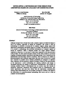
A diagram of the Watt steam engine speed control (governor) is shown in Figure 1.1. As the engine speeds up, the flyballs spin outward, moving the linkage so as to close the steam valve and thus slow the engine.

Steam Valve

Linkage Steam Engine

LOAD Main Shaft

Figure 1.1 The Watt Speed Governor 1.3 Mechatronic System Organization The developments in electronics have made it possible to energetically isolate the four components making up a controlled mechanical system, Figure 1.2. Other Components communications

Operator Interface human factors

Computation software, electronics Instrumentation energy conversion, signal processing

Actuation power modulation, energy conversion

Target System mixture of: mechanical, fluid, thermal, chemical, electrical

Figure 1.2 Mechatronic System Elements Once isolated from the instruments on one side and the actuators on the other, computation could be implemented using the most effective computing medium, independent of any needs to pass power through the computational element. That medium has been the digital computer, and the medium of expression for digital computers is software. This ability to isolate is recent. Watt’s speed governor, for example, combined the instrument, computation and actuation into the flyball element. Its computational capability was severely limited by the necessity that it pass power from the power shaft back to the steam valve. Other such examples, where computation is tied to measurement and/or actuation, include automotive carburetors, mastered cam grinders, tracer lathes, DC motor commutation, timing belts used in a variety of machines to coordinate motions, rapid transit car couplings (which are only present to maintain distance; cars are individually powered), and myriads of machines that use linkages, gears, cams, etc., to produce desired motions. Many such systems are being redesigned with software based controllers to maintain these relationships, with associated improvements in performance, productivity (due to much shorter times needed to change products), and reliability. 1.4 Amplifiers and Isolation The development of electronic amplification tachniques opened the door to mechatronics. Operational amplifier (op-amp) based circuits, such as that shown in Figure 1.3, could provide both isolation and generation of a wide variety of linear and nonlinear, static and dynamic computing functions.

Copyright © 1995, 96,97 D.M. Auslander

2

Figure 1.3 Operational Amplifier; Computing Configuration Figure 1.4 shows an alternate operational amplifier configuration, which provides even stronger isolation, but cannot perform as flexible computation.

Figure 1.4 Operational Amplifier; Follower Configuration Developments in power electronics provided the same kind of flexibility and isolation on the actuation side that op-amps provide on the signal side, and gave a means for translating commands computed in electronic form into action. Digital electronics added enormously to the range of computational functions that could be realized. Digital electronics also formed the basic technology for implementing computers, but with the use of computers it is software rather than electronics that represents the medium of expression. Although mechatronics based on electronic computing elements opened a new world of mechanical system control, software has extended that world in unimaginable ways.


3

2 Real Time Software Real time software differs from conventional software in that its results must not only be numerically and logically correct, they must also be delivered at the correct time. A design corollary following from this definition, is that real time software must embody the concept of duration, which, again, is not part of conventional software. An example showing the need of on-time delivery of results is given in Figure 2.1. In the masterless cam grinder the rotation of cam must be precisely coordinated with transverse motion to cut the non-circular cam profile. Grindstone

Cam

Figure 2.1 Masterless Cam Grinder This is an excellent example of how mechatronics can change the way that problems are approached. In a conventional, mastered, cam grinder the motion is controlled by a mechanical system which traces the contour of a master cam. The mechanical tracing mechanism must fill the role of computation (transmission of the desired contour) but also carry enough power to operate the follower mechanism. This is a limit to performance, and causes considerable loss of productivity since the time to change the machine from one cam profile to another is considerable. In the mechatronic based cam grinder, the profile is stored a an array of numbers in software, so the machine’s performance is limited only by it inherent mechanical properties. Changeover is also much faster since it only requires loading of new data. The real time software used in most mechanical system control is also safety-critical. Software malfunction can result in serious injury and/or significant property damage. In discussing softwarerelated accidents which resulted in deaths and serious injuries from clinical use of a radiation therapy machine (Therac-25), Leveson and Turner (1993) established a set of software design principles, "...that apparently were violated with the Therac-25...." Those are: - Documentation should not be an afterthought. - Software quality assurance practices and standards should be established. - Designs should be kept simple. - Ways to get information about errors -- for example, software audit trails -- should be designed into the software from the beginning. - The software should be subjected to extensive testing and formal analysis at the module and software level; system testing alone is not adequate. In particular, it was determined that a number of these problems were associated with asynchronous operations, which while uncommon in conventional software, are the heart and soul of real time software. Asynchronous operations arise from preemptive, prioritized execution of software modules, and from the interaction of the software with the physical system under control. Because of preemptive execution, it becomes impossible to predict when groups of program statements will execute relative to other groups, as it is in synchronous software. Errors that depend on particular execution order will only show up on a statistical basis, not predictably. Thus, the technique of repeating execution until the source of an error is found, which is so effective for synchronous (conventional) software, will not work with for this class of real time error.

In a like manner, there are errors that depend on the coincidence of certain sections of program code and events taking place in the physical system. Again, because these systems are not strictly synchronized, they can only have statistical characterization. 2.1 Nasty Software Properties Software complexity tends to increase exponentially with size. What starts our as a small, manageable project, can expand into something which, quite literally, never gets finished. To compound this problem, the economics of software based products is that over the lifetime of the product, maintenance costs dominate the total expense. Both the complexity and the asynchronous nature of real time software lead to situations in which bugs can remain dormant for long time periods, waiting to do their dirty work at the most inopportune time. The antidotes to these problems flow from adopting an engineering perspective so that code writing (programming) should not be viewed as a creative activity! On the engineering side, a method must be found to describe in detail how the control software should behave. This allows both for the needed engineering review function and enables the act of code production to become much more routine since the creative engineering part has been done at the descriptive level. The second way of avoiding at least some of the complexity problems is to modularize the software and its production process. In this way, specific pieces of software are directly connected to certain machine functionality. System malfunctions can thus be traced to the relevant softrware more quickly, system changes can be made with reasonable assurances that the changes will not adversely affect some unexpected part of the machine, and individual software elements can be tested more easily. 2.2 Engineering Design / Computational Performance Too often, the only detailed documentation of real time software is the program itself. Furthermore, the program is usually designed and written for a specific real time target environment. The unfortunate consequence of this is that the engineering aspects of the design problem become inextricably intertwined with the computation aspects. This situation relates directly to the first design principle listed above, "documentation should not be an afterthought." If the system engineering is separated from the computational technology, then the documentation will have to exist independent of the program; otherwise, documentation can be viewed as an additional burden. The following definitions will be used to separate these roles as they appear in the proposed methodology: System engineering: Detailed specification of the relationship between the control software and the mechanical system. Computational technology: A combination of computational hardware and system software that enables application software based on the engineering specification to meet its operational specifications. Using these definitions, the engineering specification describes how the system works; the computational specification determines its performance. As a result of this separation, if a suitable paradigm is adopted to describe the engineering specification, a much broader discussion and examination can be brought to bear because, the details of the engineering can be discussed by project participants familiar with the problem, not just those familiar with computing languages and real time programming conventions. This provides for meaningful design review of projects that are software intensive.


5

2.3 Software Portability In mechanical system control, portability has consequences both for product lifetime and for the design/development cycle. The mechanical part of the system can have a commercial lifetime of anywhere from 5 to 20 years. On the other hand, the computational technology used for its control only has a lifetime of 3 to 5 years. To remain competitive, new versions of the product need to use new computers to take advantage of the ever-increasing computational capability. Doing this cost effectively requires software that will "port" easily from the original target processor to new ones. Software portability seriously affects the design/implementation cycle as well. Early stages of the software tend to be simulations, done to test hypotheses and to substitute for hardware not yet built. Later stages use laboratory prototypes, then pilot prototypes, then, finally, the actual production system. If software can’t migrate from step-to-step in this process, the whole process can become greatly elongated as new software must be created for each step, and there are significant possibilities for introducing new bugs at each stage. Portability is complicated by the real time constraints. If real time software environments are used as aids in meeting those constraints (kernels, schedulers, real time operating systems), software written for one environment can require substantial rewriting to run in another. Crossing the full spectrum from simulation to production traverses environments in which program structure itself is incompatible. The proposed methodology provides a layer of abstraction one higher than the real time environments, so offers a means of bypassing these incompatibility problems. Further portability challenges arise from the operator interface section of the program, and the interprogram communication for those solutions implemented with multiple processors. These subjects will be discussed briefly here, but remain in need of substantial further work. 2.4 Control System Organization A two-level organization is used on both the engineering and computational sides of the control software design. On the engineering side, a job is organized into tasks states and, on the computational side, into processes threads The breakdown of the engineering specification into tasks and then states is a subjective process, requiring considerable engineering judgement. This stage is the primary creative design step. Tasks represent units of work; they are the functional subunits of the job. Tasks can often be designed by breaking a system down along both time scales and physical components. For example, there might be separate tasks to handle the high-level part of controls for several motor-driven axes, and other tasks to handle the higher speed operations associated with measurement and actuation of those same motors. Tasks, in general, are active simultaneously. They are used to describe the parallelism inherent in the physical system.


6

Internally tasks are organized in a strictly sequential manner into states. States describe specific activities within the task; only one state can be active at a time. The active state controls the current activity of the task. The primary reason for this distinction between the nature of tasks and states is that sequential activity is a part of many mechanical systems. Even for systems that do not seem to be fundamentally sequential, such as process or web systems, the sequential breakdown within tasks seems to work quite well. During normal operation, tasks tend to stay in only one or two states. However, during startup and shutdown, the task/state structure describes the operation very well. The sequential state structure also serves as one test for appropriate task definition. If tasks are aggregated to much, they will end up with parallel operations which cannot be described effectively by states. Breaking the task into several smaller tasks solves the problem. On the computational side, processes describe computational entities that do not share an address space (this includes independent processors). Threads, are computational entities that share an address space but can execute asynchronously. A thread can contain one or more tasks; a process can contain one or more threads. The organization into processes and threads is purely for performance purposes. As is noted below, there is no theoretical necessity for such organization at all. The organization serves only to meet performance specifications when the chosen processor is not sufficiently fast to meet the specs with a single-thread structure. It does this by shifting processor resources from low priority to high priority tasks. As a further note, the portability requirements enumerated above imply that several different computational organizations will be used in the course of a development project. 2.5 Task Selection in a Process System A prototypical process system is shown in Figure 2.2 (sensors are not shown).

Filler Tubes

Tank

Fluid B Fluid A

Tank

Tank

Electric heater

Electric heater

Valve

Valve

Electric heater Valve

Track

Carriage

Figure 2.2 Prototype Process System

The process contains three tanks that are used to store feedstock for a downstream process. It is necessary to maintain the composition of the liquid in each of the tanks, as well as the temperature. To assure an


7

adequate supply, the level must be maintained within certain specified limits. The outflow valves are operated by the downstream process not by the controller for this process. Liquid is delivered to the tanks with a dual feed tube, containing separate flow controls for fluids A and B. There is only one feed tube and it can be moved to whatever tank needs service by a motor. The first stage in the design of the control software for this system is the selection of tasks. A possible task list is given below. It is important to note, that this particular selection is not unique. In each case, the selection must be examined to see that the desired operating modes can be attained and that tasks do not encompass too many functions making them overly complex. Name

Function

Master OpInt Position Motion Level Pumps Temp1 Temp2,3

controls start-up, operating mode, shutdown operator interface position control of carriage gives setpoints to ‘Position’ to assure smooth motion monitors and controls liquid level and mixture controls flowrate through pumps controls tank1 temperature ...

Some tasks are simple and have very little internal structure. Others are more complicated. A method of notating internal task structure is necessary to provide sufficient modularity. This is done with the state specification.


8

3 State Transition Logic The task organizational structured described in this paper is an adaptation of state transition logic (Auslander, 1993a). This adaptation provides for implementation of the structural principles enumerated above. Documentation development is integrated with the software specification procedure, the software produced is inherently modular, and audit trail information can be produced automatically. By extending the transition logic paradigm to cover the entire realm of real time requirements (Auslander, 1993b), two important results are achieved: 1) The discipline associated with following a formal design paradigm is extended to the "low level" as well as high level software tasks. 2) It becomes possible to produce portable code, that is, code which can be generated and compiled to run in a number of different real time environments without changing the userwritten portion of the code. State transition logic is formally defined within finite automata theory (Kohavi, 1970). As used in the design of synchronous sequential circuits, it becomes a formal, mathematical statement of system operation from which direct design of circuits can be done (Sandige, 1990, or any basic text on logic design). When used as a software specification tool, state transition logic takes on a more subjective cast; the transition logic specifies overall structure, but specific code must be written by the user (Dornfeld et al, 1980, Bastieans and Van Campenhout, 1993). The state transition logic concept has been further specialized to mechanical system control through the specification of a functional structure for each state. This structure specifies the organization of code at the state level so that it corresponds closely with the needs of control systems. The use of transition logic has also been based on the very successful applications of programmable logic controllers (PLCs). These devices, in their simplest form, implement Boolean logic equations, which are scanned continuously. The programming is done using ladder logic, a form of writing Boolean equations that mimics relay implementation of logic. In basing real time software design on transition logic, each state takes on the role of a PLC, greatly extending the scope of problems that can be tackled with the PLC paradigm. Depending on the nature of the problem being solved, other formulations have been proposed. For example, the language SIGNAL (Le Guernic et al, 1986) was invented for problems which have signal processing as a core activity. Benveniste and Le Guernic (1990) generalize the usage to hybrid dynamical systems. 3.1 States and Transitions State specifies the particular aspect of its activity that a task is engaged in at any moment. It is the aspect of the design formalism that expresses duration. States are strictly sequential; each task is in one state at a time. Typical activities associated with states are:

! !

Moving - a cutting tool moving to position to start a cut, a carriage bringing a part into place, a vehicle holding a velocity. Waiting - for a switch closure, for a process variable to cross a threshold, for an operator action, for a specified time.

!

Processing - thermal or chemical processes, material coating in webs.

!

Computing - where to go, how long to wait, results of a complex measurement.

!

Measuring - size of a part, location of a registration mark, object features from vision input, proximity.

Each state must be associated with a well-defined activity. When that activity ends, a transition to a new activity takes place. There can be any number of transitions to or from a state. Each transition is associated with a specific condition. For example, the condition for leaving a moving state could be that the end of the motion was reached, that a measurement indicated that further motion was not necessary, that an exception condition such as stall or excessively large motion error occurred, etc. 3.2 Transition Logic Diagrams State transition logic can be represented in diagrammatic form. Conventionally, states have been shown with circles, and transitions with curved arrows from one state to another. Each transition is labelled with the conditions that specify that transition. This format is inconvenient for computer-based graphics, so a modified form, shown in Figure 3.1, is used. time-out

Move to Loading Position

at loading position Wait to be Loaded

load in place

Figure 3.1 Fragment of a Transition Logic Diagram

This diagram shows a fragment of the transition logic for a task that controls the movement of a materials handling vehicle. The vehicle moves from one position to another, picking up parts in one position and dropping them off at another. The states are shown with rectangles; a description of the state is given inside the rectangle. The transitions are shown with arrows and the transition conditions are shown inside rounded rectangles. The dashed lines provide an unambiguous indication of which transition the condition is attached to. The first "move-to" state shows a typical normal transition as well as an error transition, in this case based on a time-out condition. Although these diagrams are not essential in using transition logic, they are an excellent visualization tool. If a task is compact enough to fit a logic diagram on a single page, the graphical description makes its function much easier to grasp. 3.3 Tabular Form for Transition Logic The state representation of a task does not have to be graphical. Complicated tasks can have diagrams that are difficult to read and it can be difficult to automate the process of producing the diagrams from a computer. Tabular representations can give the same information and, in some cases, are easier to deal with than diagrams. A general form for representing a state is:


10

State Name [descriptive comment] - transition target #1; reason for transition [comment] - transition target #2; . . . For the transition logic fragment shown in Figure 3.1, the tabular form could be shown as: Move to Loading Position [move the cart] - Wait to be loaded; if at loading position - Xxxxxxx; if time-out Wait to be Loaded [hold cart in position until loaded] -Yyyyyy; if load in place This format is equivalent to the diagram and more compact. For some people it may be more readable, for others, less. 3.4 Example: Pulse-Width Modulation (PWM) Pulse-width modulation is widely used as an actuation function where there is need for a digital output to the actuating device, but continuous variation in the actuator output is desired. Anytime the actuator plus target system constitute a low-pass filter, PWM can perform the function of a digital-to-analog converter by exploiting the termporal properties of the low-pass filtering. The PWM signal is usually a retangular-wave of fixed frequency, with variable duty-cycle (i.e., ratio of on-time to cycle time). The logic diagram in Figure 3.2 shows a task to implement PWM and a typical PWM signal is shown in Figure 3.3.

PWM_ON START

end of on-time && duty-cyle == 1

end of on-time && duty-cycle < 1

INITIALIZE_PWM set duty-cycle to zero

PWM_OFF COMPUTE_TIMES compute on/off times based on current duty-cycle

end of off-time

duty-cycle > 0

duty-cycle == 0

Figure 3.2 Transition Logic for Pulse Width Modulation The task has four states, as shown, and will produce an effective low frequency PWM from software. The maximum frequency depends on the means of measuring time that is utilized, and the timing latencies encountered in running the task. It would be suitable for actuation of a heater or, perhaps, a large motor, but would be too slow for a modest sized motor.


11

50% Duty Cycle

25% Duty Cycle

Figure 3.3 Pulse Width Modulation: Two Duty Cycles

The two main tasks, PWM_ON and PWM_OFF, turn the output on (or off) on entry, and then just wait for the end of the specified time interval. COMPUTE_TIMES is active once per cycle to find the appropriate on and off times in the event that the duty cycle has been changed. The transition conditions take account of the two special cases -- duty cycles of 0 (never on) and 1 (always on) in addition to normal operation. This example shows the use of transition logic for a task that is quite low level computationally. Unlike a conventional implementation of such a task, however, the details are readily apparent from the transition logic and reference to the code (not shown here) need only be made to confirm that it accurately translates the transition logic. 3.5 Transition Logic for the Process Control Example The process system of the previous chapter is repeated in Figure 3.4. The control objective is to maintain the mixture, temperature and level in each of the tanks.

Filler Tubes

Tank

Fluid B Fluid A

Tank

Tank




Track

Carriage

Figure 3.4 Prototype Process System Of the tasks defined for this system, the level task is probaably the most complex. Its job is to figure out which tank needs attention at any time, ask for carriage motion, and initiate the filling action. The transition logic for this task is shown in Figure 3.5.


12

Start [wait for OK to start]

OK

Monitor [Determine which tank (if any) needs service]

tank3

tank1 tank2

Move1 [send command to move filler to tank1] at tank1 Pump1 [initiate pumping with specified mixture] filled

Move2 [send command to move filler to tank2]


at tank2 Pump2 [initiate pumping with specified mixture] filled


Figure 3.5 Transition Logic for the Level Task This task functions largely in a supervisory role. It examines the current status of each of the tanks, and then sends out commands to provide the service it deems necessary. Other tasks are responsible for actually carrying out those commands. This state diagram is typical of the level of detail that is used. The Monitor state is identified as determining which tank needs service. How this is determined is not specified in the state diagram. That is a well defined function, and should be specified in the auxiliary documentation accompanying the state diagram (or tabular state representation). When code for this function is written, there will be a very clear path indicating when and how the code is used, and an explanation of what the code should be doing. Other states are simpler, and probably do not need much if any auxiliary documentation. 3.6 Non-Blocking State Code A major feature of programmable logic controllers (PLCs) contributing to their success as industrial control components has been that the logic function is continually scanned. The programmer does not deal with program flow control, as must be done when using conventional programming languages. As long as the ladder is active, it is scanned repeatedly, so the user only has to be concerned with the fundamental performance issue of whether the scan rate is adequate for the particular control application (PLCs are programmed in a form of logic notation called ladder diagrams). Transition logic design is based on this same scanning principle for execution of state-related code. In order to achieve greater functional flexibility than is possible with ladder diagrams, however, standard sequential languages are used for coding. To implement a scanning structure with algorithmic languages requires the restriction that only non-blocking code can be used. Non-blocking code is a section of program that has predictable execution time. The execution time for blocking code cannot be predicted. This definition does not say anything about howlong that execution time is. For now, it is enough that it be predictable. How long the execution time is for any specific piece of code is a performance issue and will be dealt with later.


13

Examples of blocking code in the C language include, for example, the scanf() function call used to get keyboard input from the user. Scanf only returns when the requested input values have been typed; if the user goes out for coffee, the function simply waits. Likewise, the commonly used construction to wait for an external event such as a switch closure, while(inbit(bitno) == 0) ; is also blocking. If the event never happens, the while loop remains hung. This restriction to non-blocking code does not cause any loss of generality at all. Quite the contrary, the transition logic structure is capable of encoding any kind of desired waiting situations, as shown in the examples given above. By encoding the "wait" at the transition logic level rather than at the code level, system operations are documented in a medium that any engineeer involved in the project can understand without having to understand the intricacies of the program. 3.7 State-Related Code The transition logic metaphor encourages the use of modular software by associating most of the userwritten code with states. Although this level of organization is adequate for simple projects an additional level of organization is necessary in most cases. To this end, an additional formal structure of functions is established for the state-related code. Two goals of modular code writing are thus fulfilled: a) Sections of code are directly connected to identifiable mechanical system operations, b) Individual functions are kept short and easily understood. These functions are defined around the operational assumption of a scanned environment -- the code associated with a state is “scanned,” that is, executed on a repeated basis, as long as that state is the current state for a task. Code associated with non-current (inactive) states is not executed at all. For each state, the following functions are defined: Entry function: Executed once on entry to the state. Action function: Executed on every scan of the state. For each transition from the state, the following pair of functions is defined:

Test function: Test the condition for transition; returns TRUE or FALSE. Exit function: Executed if the associated transition is taken. This structure enforces programming discipline down to the lowest programming level. All of these functions must be non-blocking, so, test functions, for example, never wait for transition conditions. They make the test, then return a logic value. Relating code to design-level documentation is also enforced with this structure. Transition logic documentation for each task identifies states in terms of what the mechanical system is doing. Not only is the code relevant to that state immediately identified, the code is further broken into its constituent parts. 3.8 State Scanning: The Execution Cycle The state scan is shown in Figure 3.6. In addition to establishing the execution order for the state-related functions, it also provides the basis for parallel operation of tasks.


14

Each pass through the cycle executes one scan for one task. If this is the first time the scan has been executed for the current state, the entry function is executed. The action function is always executed. Then, the first transition test function is executed. If it returns TRUE to indicate that the transition should be taken, the associated exit function is executed and a new state is established for the next scan. Otherwise, subsequent test functions are executed in a similar manner. The first test function returning TRUE terminates the sequence. Thus, if more than one transition became TRUE at the same time, the one associated with the earliest test function would be recognized. Behind the execution details, there must be a data base of task information. Each task must have a data table specifying its structural information, that is, all of the states and transitions, task parameters such as priority, sample time, etc., and the transient information such as present state and status. 3.9 Task Concurrency: Universal Real Time Solution Tasks, as noted above, must operate concurrently. This structure provides for parallel operation of tasks, even in the absence of any specific multitasking operating system or dispatcher. Because all of the state functions are non-blocking, the scan cycle itself is non-blocking. It can, therefore, be used to scan each active task in succession. After finishing with all of the tasks, the first task is scanned again. This guarantees fully parallel operation of all tasks.

Start Entry to state ?

Yes

No

Execute entry function

Execute action function

Execute first test function

Yes

True ? No

... (other transition tests)

Execute exit function

Set new state and set state entry flag

Done

Figure 3.6 State Scan Cycle

This method of dispatching, cooperative multitasking, will be an adequate solution if the total scan time for all tasks is short enough to meet the system timing constraints (the term scheduling is often used synonymously with dispatching; in this material scheduling will usually be used for a planning activity concerned with meeting execution time targets while dispatching will be used for the part of the program that actively directs task execution). If cooperative multitasking is not adequate, a faster computer must be used, or other dispatching solutions must be found. These will be discussed below. The methodology discussed thus far therefore presents a universal real time solution. It is capable of solving all real time problems, without any special real time constructs or operating systems, if a fast enough computer is available. All of the usual real time facilities, semaphores, task synchronization, event-based scheduling, etc., can all be implemented using the formalism of transition logic, with all code non-blocking. If a fast enough computer is not practical, use of preemptive dispatching based on interrupts can be implemented. To do this, the transition logic paradigm must be extended to include designation of tasktype, and library code must be included to allow integration of transition logic based code with a variety of real time and/or multiprocessor environments.


15

4 Direct Realization of System Control Software The task and state specification for a project, along with the auxiliary documentation should constitute a complete engineering specification for the operation of a mechatronic control system. The realization stage of the project is the translation of the specification into computer code. The computer code is ideally constructed independently of specific computational environments. It is ideal in the sense that choice of language and level of code formality will have an effect on computational environments into which the code could be ported. For example, if the language C is chosen to prototype a problem that will ultimately be implemented in a minimally equipped microcontroller, the final production code may well not be in C. Even in these situations, however, because the primary technical description of what the code does is in the task/state specification, code translation from one realization to another should be relatively simple. This chapter will deal with realization of the code using the simplest level of formality and implementation of that code in the simplest possible computational environments -- those that provide at most the ability to tell time but do not support any form of preemptive execution. It is the first step in specification of a method of dispatching based on tasks which are grouped according to priority. The only facilities expected are a compiler for the target language and an operating environment to run the program. 4.1 Language Computer languages are the source of fierce debate among their devotees. While many of these debating points have considerable merit, the approach taken here is that the important information lies in the abstraction level above the code, so that the particular choice of language is more a matter of convenience and access. A wide variety of implementations are possible once the task/state description is done. Depending on the complexity of the problem and the stage in the design process, the implementation might be done in a relatively informal manner, or could be accomplished in a formally defined environment. The software tools available will also vary widely. For that reason, sample solutions are presented in one or more of two-and-one-half languages. The simplest implementations environment from the language point-of-view use Matlab. Matlab is simple from the language structure perspective, but provides a very rich environment for simulation and analysis. This is exactly what is needed for early design and feasibility stages. Matlab is highly interactive and is a good environment for debugging, but has very slow execution speed for the types of problems that are common in mechatronics. However, even at the slow execution speed, with a fast comuter it could be used for actual realization of process control systems. The other one-and-a-half languages refer to C and its superset language, C++. C is by far the most commonly used high-level language for control of mechatronic systems. C++ has additional structure beyond that of C and that structure is extremely useful in imposing a programming style that is much more effective in capturing the task/state structure used for the engineering. There will be many situations in which C++ is either not available or not used. C is thus an essential tool for control and problem solutions built with very little pre-established software structure will be illustrated using C. Because of its very strong internal structure, C++ will be utilized to build an environment in which task and state formalisms are already defined so the user has only to fill in the application specific code. The highly formal C++ solutions have the greatest degree of portability since the underlying software that connects the user code to the computational environment can be treated as a utility and need only be written once for each environment. The application code does not need to change at all. On the other hand, a full C++ compiler is necessary in each target environment. The less formal solutions, usually implemented in C, require more change for porting, but only require a C compiler or, sometimes, no more than a subset-C-compiler.

Implementation in almost any other language is possible. It should be easy to translate the examples in Matlab, C or C++ into almost any language, including assembly language. Code for short programs or fragments of longer programs will be shown in the text. Full source code is available from the archive collection of all of the examples and utility code. 4.2 Time Almost all mechatronic control programs need access to explicit values of time. In the direct implementations described in this chapter all of the decisions tasks need to make about time are done explicitly, within the task. These calculations definitely need to be able to know the current time. Within the control elements of the program as well, time is often explicitly used, for example, in scheduling or dispatching a certain amount of time to a particular operation. Simulation programs only need their internal, “simulated” time. There is no real time. The simplest way of generating real time for actual realizations of control programs is through calibration. This requires no specific computer hardware or software utilities at all. It is accomplished by establishing an internal program variable for time, and incrementing that variable at a fixed spot in the program (much as is done in a simulation program). Calibration is done by running the program for a long enough time to exercise as much as possible of its functionality and for a long enough time to get a reliable measure of actual run time. The value by which time is incremented each pass is then adjusted so that the program’s internal time matches real time. This method is not very accurate, but it is extremely simple to implement. It is quite good when what is needed is a medium scale knowledge of time, but high accuracy is not required for either very short or verylong time periods. The calibration must be redone whenever the program is run on a different processor, or whenever the program is changed. The calibration is very easy to do, however. To go beyond the accuracy available with the calibrated method, an actual physical clock must be used. This normally consists of a highly stable crystal oscillator whose output drives a counter. Details of how the clock is implemented will be presented in a later chapter. For the purposes of this chapter, it is assumed that the current time is always available via a function call. That time value will normally be a measure of the time since the program was started, but sometimes the scale will have an arbitrary origin. 4.3 Program Format As a means of organizing control programs, the suggested format is that each task be represented by a separate function and, where possible, each task’s function is in a separate file. This assures maximum portability and makes it easy to match code to documentation. State-based code, action, entry, test and exit functions, can be either in-line or defined in separate functions, depending on their complexity. In addition to the task-related code, there is usually some form of “main” function that is used to set the program up, initialize variables, etc., then start the control operation. The form that this section takes depends strongly on the specific environment. 4.4 Simulation Simulation provides an extremely valuable environment for the initial testing and debugging of control programs. Themost important aspect of using a simulation is that the basic software can be tested in an environment that is convenient and efficient to use and in which it is relatively easy to find bugs. The


17

simulation environment is a conventional, strictly synchronous computation environment so errors can normally be reproduced by running the program again. This is often not the case when the control is operated in its target environment because the control program and the target physical system operate asynchronously. It is very tempting to skip the simulation step in system development and go straight to lab prototype. The temptation arises because it takes significant resources to construct the simulation. Would these resources be better used for the lab prototype? In general, no. Debugging in the simulation environment is so much more efficient than in the prototype environment that the investment in a simulation pays off rapidly. 4.5 Simulation in Matlab All of the files referred to in this section are found in the archive file grp_mtlb.zip. The “grp” refers to these program being part of the group priority method of program construction. The zip file contains directories for each of the examples. 4.5.1 Template for Simulation Using Matlab (grp_mtlb.zip, directory template) This template gives a model for direct implementation of the task/state model of control systems. “Direct” indicates that no software base is used in building the control program other than the language facilities themselves. The model is thus applicable to virtually any computing environment and any computing language. Matlab is a convenient environment for simulation, and the language is simple enough so that the results can easily be translated to any other desired target language. This section will thus serve as a template for applications in any language other than C or C++. As computer speeds increase, Matlab itself could become a convenient real time environment for prototyping; otherwise a translation must be done before control of theactual target system can be accomplished. The template below is in two parts. The first part is the initialization and runtime control portion of the program. This is done here as a Matlab script file, although it could be implemented as a function as well. The primary control loop has three major parts: the output section, the execution of the tasks, and the simulation of the continuous-time part of the problem. The other part of the template is the task file. It shows the structure of a typical task. Each task would have a file matching the template in form. Note that in some cases the word processor will wrap long lines in the listing to a second line. This could result in line fragments that are not syntactically correct -- for example, comments that have been wrapped put the last part of the comment on a line with no comment indicator (% in Matlab). Initialization and Runtime Control % Template for Matlab mechatronics control programs % This template is for a single-thread, sequential scheduler % File:tpl_seq.m % Created 8/1/95 by DM Auslander

glbl_var % Read in global definitions -- because each function %in Matlab requires a new file, this is a more compact %way to share variables % System setup and initialization % Put initial values for all variables here % Simulation parameter values tfinal = 30;


18

del_t = 0.2; % Simulates the minimal increment of computing time ept = del_t / 100; % Used to check for round-off errors del_tsim = 0.6; % Simulation discretization interval. Must be >= del_t % Use this to control the number of output values t_outint = 0.5; % Time interval for outputs. Usually greater than del_t % This is particularly important for the student edition! nouts = ceil(tfinal / t_outint); yout = zeros(nouts + 1,4); % Set this up for proper output dimension tout = zeros(nouts + 1,1); t_outnext = 0; % Time at which next output will be copied iout = 1; % Index for outputs tstep = 0; % Running time % Set up the options for the differential equation solver % (if one is being used). % Several simulation options are possible. Odeeul is a function % that does a one-step Euler integration. It is very efficient, but very % dangerous mathematically because it has absolutely no error control % Another good option is to use the functions in Odesuite, a new % Matlab integration package. The version used here has been modified % with a parameter ’hfirst’ so it can be used more efficiently in this % hybrid (discrete-time/continuous-time) environment. ode_opts = odeset(’refine’,0,’rtol’,1.e-3); % Differential solver options % ’refine’ = 0 causes the ode solver to output only at the end % Make up a task list using the string-matrix function, str2mat() % Note that this can only take 11 strings in each call, so it must be called % multiple times for more than 11 tasks % Each name represents a function (file) for that task t1 = str2mat(’task1’,’task2’,’task3’); tasks = str2mat(t1); nn = size(tasks); ntasks = nn(1); % Number of rows in ’tasks’ % Set initial states Stask1 = 0; % A state of 0 is used as a a flag to the Stask2 = 0; % state to do whatever initialization it needs Stask3 = 0; % Also set up the state vector for ode simulation here if one is being used % Initialize all the tasks for j = 1:ntasks tsk = tasks(j,:); % name of j-th task feval(tsk); % No arguments - task takes care of state % and when it runs internally. end i_audit = 1; % Index for transition audit trail tbegin = get_time; % Time at the beginning of simulation step % Step out the solution while tstep = t_outnext t_outnext = t_outnext + t_outint;% Time for next output yout(iout,1) = out1; yout(iout,2) = out2; yout(iout,3) = out3; yout(iout,4) = out4; tout(iout) = tstep; % Record current time iout = iout + 1;


19

end % Run the control tasks for j = 1:ntasks tsk = tasks(j,:); % name of j-th task feval(tsk); % No arguments - task takes care of state % and when it runs internally. inc_time; % Increment time del = get_time - tbegin; % Time since last simulation if del >= del_tsim % If true, do a simulation step tbegin = get_time; [tt,xx] = odeeul(’proc_sys’,del,x,ode_opts); x = xx; % Update the state vector end end tstep = get_time; % Update time end % Record the final output values yout(iout,1) = out1; yout(iout,2) = out2; yout(iout,3) = out3; yout(iout,4) = out4; tout(iout) = tstep; % Last recorded time

The most important part of this template is the loop that executes the tasks, for j = 1:ntasks tsk = tasks(j,:); % name of j-th task feval(tsk); % No arguments - task takes care of state % and when it runs internally. inc_time; % Increment time del = get_time - tbegin; % Time since last simulation if del >= del_tsim % If true, do a simulation step tbegin = get_time; [tt,xx] = odeeul(’proc_sys’,del,x,ode_opts); x = xx; % Update the state vector end end

For each pass through the major loop, this inside loop will cause all of the tasks to be executed once, thus implementing the basic multitasking. This is considered the basic unit of computation, so the simulated time is incremented for every scan. Execution of the simulation is also done inside this loop. To improve efficiency a bit, the simulation can be executed on a longer time scale than once every minimal time step. The ODE-solver shown here is an extremely simple one-step Euler integrator. It was written specifically for these applications, since the basic time step unit for control is often small enough for the Euler integrator to be effective. It is not a general-purpose integration function. Intergration routines based on a modified version of the Matlab ode-suite are used in other examples. For each task, this scan will cause execution of the state code associated with the current state for that task, as shown below. Template for a Task function task1 % Template for a typical task function (which has to be % a separate file with the same name in Matlab) glbl_var

% Global definitions


20

% The ’next-state’is maintained as a separate variable so that the % initialization canbe handled correctly and so a test can be % constructed to tell whether the entry function of a state % should be run. The next-state variable must be static so it % remembered across function invocations. The ’global’ designation % is the only way Matlab has of making a variable static. % The default value of the next-state variable is -1, indicating % that no state change has taken place. global S_task1_next % Next state for this task (other local statics % can be listed here). % These aren’t really global, but do have to be ’static’ % Matlab doesn’t have a ’static’ declaration so this will have to do! if S_task1 == 0 % Initialization section - occurs once only S_task1 = 1; % Make sure this section is not executed again! S_task1_next = 1; % First state. %The default is -1 which indicates stay in same state return; end % This task runs at specific times. If current time has not reached % the scheduled run time, just return. if tstep < Ttask1 return; end Ttask1 = Ttask1 + Tdelta; % Time for next run -- in this case % the task runs at regular intervals, but that needn’t % be true all the time. if S_task1_next ~= -1 % There has been a state change (including self-transition) [i_audit,trans_trail] = audit(2,S_task1,S_task1_next,... tstep,trans_trail,i_audit); % Record this transition S_task1 = S_task1_next; run_entry = 1; S_task1_next = -1; % Default - stay in same state else run_entry = 0; end % Run the code associated with the current state if S_task1 == 1 % Entry section if run_entry % Only run this on entry to the state % code for entry section goes here (if any) end % Action section % code for action section goes here (if any) %Test/exit section if s1_test % Test for first possible transition % this could be a separate function or % in-line code. % A new state has been requested S_task1_next = 2; % Specify the next state % Exit section % code for exit section (if any) end


21

% Similar code goes here for additional transitions % associated with this state. % Code for another state elseif S_task1 == 2 % ... Repeat this pattern for as many states as there are % in this task

else % Check for a state variable value that doesn’t % correspond to a defined state. error(’Task: Task1 -- unknown state encountered’); end

Every time a transition between states is detected, a call is made to the audit function. This keeps track of all the transitions. The audit function is (line breaks in the first line have been inserted by the word processor!): function [i_audit,trans_trail]=audit(task,from_state,to_state,time,trans_trail,i_audit) % Record state transitions i = i_audit; trans_trail(i,1) = time; trans_trail(i,2) = task; trans_trail(i,3) = from_state; trans_trail(i,4) = to_state; i_audit = i_audit + 1;

4.5.2 Simulation of PWM Generator (grp_mtlb.zip, directory: pwm_samp) The Matlab templates given above are used to build a simulation of the PWM generator introduced earlier. The simulation includes two tasks: one task that produces a command signal specifying the desired duty cycle and a second task that generates the PWM itself. The first task is very simple, and has only a single state. The second, the PWM generator, has the state structure in Figure 4.1 (repeated from previous chapter). Excerpts of the code for this sample are shown below.

The main script file follows the template model very closely and will not be displayed here. This simulation generates the PWM signal, but has no target system. It thus does not utilize the ODE functions. The command task has only one state. That state computes a sinusoidal duty cycle command signal. The code for its sole state is:

PWM_ON START

end of on-time && duty-cyle == 1

end of on-time && duty-cycle < 1

INITIALIZE_PWM set duty-cycle to zero

PWM_OFF COMPUTE_TIMES compute on/off times based on current duty-cycle

end of off-time

duty-cycle > 0

% This task has only one state -- it produces a command duty cycle as % a function of time. duty-cycle == 0

% Run the code associated with the current state if Spwm_cmd == 1 % Entry section % No entry section for pwm_cmd


Figure 4.1 Transition Logic for Pulse Width Modulation

22

% Action section duty_cycle = 0.5 * sin(tstep * 2 * pi / cmd_period) + 0.5; % Result is in range 0->1 %Test/exit section % This task has only one state - no transitions!

The PWM generator task follows the state diagram very closely. The only minor difference is that the INITIALIZE_PWM state is absorbed into the initialization section. The code for the this follows: if Spwm_gen == 1 % **Compute_Times** % Entry section if run_entry % Only run this on entry to the state % code for entry section goes here (if any) duty_cycle = limitval(duty_cycle,0,1); end_on_time = duty_cycle * pwm_period + tstep; end_off_time = pwm_period + tstep; end % Action section % code for action section goes here (if any) % No action function for this task %Test/exit section if duty_cycle > 0 Spwm_gen_next = 2; % Transition to PWM_On % Exit section % code for exit section (if any) % No exit section for this transition elseif duty_cycle = end_on_time) & (duty_cycle < 1) Spwm_gen_next = 3; % Transition to PWM_Off % No exit section for this transition elseif (tstep >= end_on_time) & (duty_cycle >= 1) Spwm_gen_next = 1; % Transition to Compute_Times % No exit section for this transition end elseif Spwm_gen == 3 % **PWM_Off** % Entry section if run_entry % Only run this on entry to the state % code for entry section goes here (if any) pwm_out = 0; % Turn on the PWM output end % Action section % code for action section goes here (if any) % No action function for this task %Test/exit section if tstep >= end_off_time


23

Spwm_gen_next = 1; % Transition to Compute_Times % No exit section for this transition end else % Check for a state variable value that doesn’t % correspond to a defined state. fprintf(’Uknown state: %f\n’,Spwm_gen); error(’Task: pwm_gen -- unknown state encountered’); end

Running this simulation produces the results shown in Figure 4.2. The top graph shows the duty cycle command, which is the product of the command task. The bottom graph shows the PWM signal.

As the duty cycle rises, the proportion of the time that the output spends at its high value increases. The frequency of the signal remains constant.

Duty Cycle

1

0.5

0 0

2

4

6

8

10

2

4

6

8

10

PWM_Out

1

0.5

0 0

Time

One of the major validation and debugging tools associated with the use of state logic is the transition audit trail that is produced. AS noted above, the array constituting the audit trail comes from the calls to the audit function embedded in the task functions. For example, the function call from the PWM generation task looks like: [i_audit,trans_trail] = audit(2,Spwm_gen,Spwm_gen_next,tstep,.. . trans_trail,i_audit);

Figure 4.2 PWM Test Results The first argument is the task number, so the task associated with the transition can be identified. The next two give the from state and the to state, followed the time of the transition, the array to store the audit information, and then the array index. The audit trail from the PWM simulation follows. The first two transitions correspond to the initialization process (at time = 0). Following that, it can be seen that all of the transitions refer to task #2, the PWM generation task. This is because task #1, the command task, has only one state and thus no further transitions. The entry at time=0.12 is the transition from state 1 (Compute_times) to state 2 (PWM_On). This is followed by a transition to state 3 (PWM_Off) and 0.62 and then a transition back to state 1 (Compute_times) at time=1.12. Since the time difference between these transitions is each 0.5, the output at that point is a 50% duty cycle, which can be confirmed from the graph. Although the numbers-only format is not the easiest to read, Matlab does not have very sophisticated texthandling functions so this is a reasonable compromise. trans_trail = (Time Tass

From-state To-state)


24

0 1.0000 1.0000 1.0000 0 2.0000 1.0000 1.0000 0.1200 2.0000 1.0000 2.0000 0.6200 2.0000 2.0000 3.0000 1.1200 2.0000 3.0000 1.0000 1.2200 2.0000 1.0000 2.0000 2.0200 2.0000 2.0000 3.0000 2.3200 2.0000 3.0000 1.0000 2.4200 2.0000 1.0000 2.0000 3.4200 2.0000 2.0000 3.0000 3.5200 2.0000 3.0000 1.0000 3.6200 2.0000 1.0000 2.0000 4.6200 2.0000 2.0000 3.0000 4.7200 2.0000 3.0000 1.0000 4.8200 2.0000 1.0000 2.0000 5.6200 2.0000 2.0000 3.0000 5.9200 2.0000 3.0000 1.0000 6.0200 2.0000 1.0000 2.0000 6.5200 2.0000 2.0000 3.0000 7.1200 2.0000 3.0000 1.0000 7.2200 2.0000 1.0000 2.0000 7.3200 2.0000 2.0000 3.0000 8.3000 2.0000 3.0000 1.0000 8.4000 2.0000 1.0000 2.0000 8.5000 2.0000 2.0000 3.0000 9.4000 2.0000 3.0000 1.0000 9.5000 2.0000 1.0000 2.0000 9.8000 2.0000 2.0000 3.0000

4.5.3 Simulation of Three-Tank Process System (grp_mtlb.zip, directory: proc_sys) The three-tank process system is more complicated than the PWM system since it encompasses more layers in the typical control system hierarchy. It also has some interesting decision-making since the filler nozzles have to be moved from tank-to-tank. The code is too long to be repeated here, so only excerpts will be given. The diagram of the system is repeated below, showing the tanks and the filler carriage, Figure 4.3. Fluid B Fluid A

Filler Tubes

Tank

Tank

Tank



Figure 4.3 Prototype Process System (repeated)


Valve

Track

Carriage

25

Electric heater

The Matlab simulation uses three tasks (the heater controls are not yet simulated), 1. Carriage position feedback control 2. Carriage motion supervisory control 3. Tank level and concentration control The Matlab simulation also does not have any operator interface, which is common of simulations. The state diagram of the level control task was already given, and is repeated here, Figure 4.4

Start [wait for OK to start]

OK

Monitor [Determine which tank (if any) needs service]

tank3

tank1 tank2

Move1 [send command to move filler to tank1] at tank1 Pump1 [initiate pumping with specified mixture] filled





Figure 4.4 Transition Logic for the Level Task

The “Monitor” state is the most interesting one in the “Level” task. It decides how to make use of the filler carriage, which is a singular resource for the system. It then sends commands to the tasks that perform the actual actions. As such, it is a form of supervisory task also since it determines setpoints and commands for other tasks. The code that implements the Monitor task is: if Slevel == 1 % Monitor % Figure out which tank needs service % Needing service is determined by the tank with the lowest level % Service is needed if the lowest level is less than (high + low)/2 % No entry section % No action section % Test/exit section imin = 1; hmin = h1; if h2 < hmin, imin = 2; hmin = h2; end if h3 < hmin, imin = 3; hmin = h3; end if hmin < (hhigh + hlow) / 2 % A tank needs filling if imin == 1, slevel_next = 2; % to Move1 elseif imin == 2, slevel_next = 4; % to Move2 elseif imin == 3, slevel_next = 6; % to Move3 end end Copyright © 1995, 96,97 D.M. Auslander

26

A very simple decision algorithm is used here: if any tanks are below their specified mean heights (in this case, the same for all tanks), those tanks are serviced in numerical order. Furthermore, no other tanks are serviced until the tank currently being serviced has reached its specified height. The carriage-motion task is the other supervisory task. Its purpose is to generate setpoints to the position control task so that the motion of the carriage will be smooth. In this case, this is done by generating a trapezoidal motion profile -- constant acceleration, followed by constant velocity, followed by constant deceleration. The state logic for this is shown below, in tabular form: Wait for Next Move [do nothing until a command is received] - Accelerate if motion command rec’d Accelerate [Constant accel to cruise velocity] - Decelerate if stop distance reached; [a short move will not have any cruise section] - Cruise if cruise velocity is reached Cruise [Maintain constant velocity] - Decelerate if stop distance reached Decelerate [Constant decel to stop] - Wait for next move if velocity reaches zero A typical move contour is shown in Figure 4.5 The velocity has sharp corners when moving in and out of Cruise, but the position curve is smooth. This profile is satisfactory for many move profiles, but still smoother (jerkless) profiles can be generated if necessary. Path Distance and Velocity

The effect of the motion supervisory task is seen in the smooth transition of the carriage from moving to stopped.


Path Distance

1.5 1 0.5 0

0

1

2 Time

3

4

0

1

2 Time

3

4

0.6 Path Velocity

A typical simulated system performance is shown in Figure 4.6. The top set of lines is the height of liquid in each of the three tanks. The bottom solid line is the position of the carraige. As long as the height in all three tanks remains suitably high, the carriage remains at its initial position (x=0). When the tank shown by the dashed line reaches a critical height, the carriage starts moving. The filling is delayed by the time the carriage is in motion. Filling starts as soon as the motion stops, as can be seen from the upward slope in the liquid height curve.

0.4 0.2 0

Figure 4.5 Trapezoidal Velocity Profile

27

Carriage Position and Liquid Levels 4.5 4 3.5 3 2.5 2 1.5 1 0.5 0

0

5

10

15 time

20

25

30

Figure 4.6 Process System Behavior

4.6 Intertask Communication Communication of information between tasks was accomplished in the Matlab environment through the use of the global definition. While this is adequate for Matab, and convenient because the Matlab environment becomes awkward if large numbers of functions are defined, it does not provide a general enough mechanism for intertask communication. The reasons for this involve both data integrity and program portability, and will be discussed in more detail in a later chapter. The mechanism for writing programs in the direct and simply structured manner used in this chapter but still preserving easy portability to more complex environments requires two steps: 1. Associating variables with tasks rather than with the whole program. 2. Explicitly identifying all information transfers between tasks. The simplest way of implementing this is for every variable in a task that is needed in other tasks, define an associated variable that is used only for transferring information. Using variable names that begin with x_ (for exchange) will help identify them quickly when looking at code. Then, for each such variable define a get_xxx() function that other tasks can use to get the value of that variable when it is needed. For efficiency, variables that are always needed as a group can share a single function. The exchange variables are set to the value of their corresponding local variables at a place in the code where the local variable has a well-defined value. For example, it is common to test a variable against a limit, x1 = .....; if(x1 < xmin)x1 = xmin; else if(x1 > xmax)x1 = xmax;

Until the end of the complete sequence, the variable x1 does not have a well defined value. In many other calculation sequences, a variable might appear several times as various intermediate values are set. Copyright © 1995, 96,97 D.M. Auslander

28

The final step is to prevent any task preemption from occurring while a data transfer is taking place. The simplest way to do this in a uniprocessor system is to disable the processor’s interrupts during the transfer, disable_interrupts(); x_x1 = x1; enable_interrupts();

This sequence should be used in any statement that either uses or sets an exchange variable, including within the get_xxx() function. The purpose of this is to insure the integrity of the transferred data by preventing interrupts from occurring in the middle of a transfer. These procedures can only be ignored in those environments that cannot implement preemptive action (such as Matlab). 4.7 Simulation in C and C++ If C is to be the target language, it makes sense to do the simulation in C also. Most of the template for direct simulation in C is very similar to the Matlab template. Unlike Matlab, some external mathematical library function for approximate integration must be added if there is a continuous-time element of the simulation for the target system. The results must be written to a file since C does not have any equivalent to the Matlab ‘workspace’ to leave the result in. 4.7.1 Template for Simulation Using C [C templates not done yet] 4.7.2 Templates for Simulation Using C++ (grp_cpp.zip, directories: template and common) The C++ template makes use of two base classes for building the application program -- one for the tasks and one to organize the task lists. These are in the file basetask.hpp. The base class for task definition, BaseTask, is quite simple. This is because in the direct program design method all of the properties of the task are embedded into the user-written task code, there is very little common information. The most important item in the base class definition is the Run function, which is declared as virtual. The actual tasks are defined by inheriting from this base class. Each task must define an actual function of this name which is where all of the state code goes. If the base class Run function is ever called it gives an error message. The other items in the class are the task name, which is used for the audit trail and anything else the user wants to use it for and some basic data that all tasks need. BaseTask is: class BaseTask { public: BaseTask(char *aName); virtual ~BaseTask(); virtual int Run(void); long GetNumScan(void); char *Name; // Task name (for debugging) int TaskID; // ID number that can be used to track tasks protected: int State, xState; // Keep track of the current State. int NextState; // The State to be run next execution scan. -1 means no change int RunEntry; // Flag set on State change to cause entry function to run double NextTaskTime, xNextTaskTime; // The next time this task should run


29

double DeltaTaskTime, xDeltaTaskTime;// Period for this task long NumScans; // For performance tracking };

There are two classes defined for list maintenance, TListElement and TList. These provide for construction of a linked list of items associated with the BaseTask class, which will be used for scheduling. They are: // TListElement - data associated with any element on a list class TListElement { public: TListElement(BaseTask *ItemPointer); ~TListElement(void); TListElement *Next; BaseTask *Item; }; // TList - a list of BaseTasks. The list allocates space // for itself as elements are added via Append. class TList { public: TList(void); ~TList(void); void Append(BaseTask *Item);// Add Item to end of list BaseTask *NextItem(void); // Return pointer to next // item on list. int IsEmpty(void); int HowLong(void);

// Is the list empty // How many items on list

private: TListElement *First; // First element on list TListElement *Last; // Last element on list TListElement *Current; // Last element on list int Length; // Number of elements on list };

The file basetask.cpp contains the functions associated with these classes. The only task-related function is the default Run function, which prints an error message. The other functions are for lists, adding and removing items, etc. The complete main file is included below. It follows the format of the Matlab version fairly closely with one significant difference: the simulation is handled as a separate task rather than built into the main execution loop. The new operator is used for most of the item creation activities. In the initialization part of the main function, new is used to set up the list of tasks, and also to set up the arrays for the output information. The execution loop has two major sections. It first checks to see if outputs should be added to the output array and then scans the list of tasks using the functions from the list processing class. Finally, after the execution loop is done, the outputs from the output data and the audit trail are written to data files. // Template for the "main" file of a group priority application // File: mainfile.cpp


30

// Created by D. M. Auslander and J. Jones, 12/19/95 // (based on existing examples) // This file shows skeletons of all of the component // parts of an application. It cannot be compiled because // the actual code is missing. It can be used to build a // program by filling in the missing pieces and changing // names (away from the generic names such as "task1") // There are also template files for the task file and for // the header file, tasks.hpp #define MAIN_CPP #include #include #include #include #include #include "tasks.hpp" // Task and environment info static StopControlNow = 0; // Variables and function used to char *StopMessage = NULL; // turn the program off void StopControl(char *aMessage) { StopControlNow = 1; StopMessage = new char[strlen(aMessage+1)]; strcpy(StopMessage, aMessage); } double EndTime = 1.0e10; // make this value visible to other function // in this file (use big number to run forever) void main(void) { double TheTime; // Running time // The task lists are instantiated here // Declaration of TList pointers are in tasks.hpp LowPriority = new TList("Low Priority"); Intermittent = new TList("Intermittent"); #ifdef ISR_SCHEDULING // These lists are only instantiated if interrupt // scheduling is used. Preemptable = new TList("Preemptable"); Interrupt = new TList("Interrupt"); #endif // ISR_SCHEDULING // Create all of the task objects used in the project Task1 = new CTask1("Task1"); Task2 = new CTask2("Task2"); ... // Other tasks // Instantiate the task that handles the operator interface // (if any) OpInt = new OperatorInterface("Oper Int"); // Define another task object for running the simulation. // This task is scheduled just as any other tasks, and is // only added to the task list if a simulation is desired. // The actual simulation code in contained in the Run() // member function of SimulationTask. // Note that this use if the #define SIMULATION is optional. #ifdef SIMULATION SimTask = new SimulationTask("Simulation"); #endif //SIMULATION


31

// All tasks must be added to the task list here. #ifdef ISR_SCHEDULING Preemptable->Append(Task1); Interrupt->Append(Task2); #else // ISR_SCHEDULING Intermittent->Append(Task1); LowPriority->Append(Task2); #endif // ISR_SCHEDULING LowPriority->Append(Task3); LowPriority->Append(OpInt); #ifdef SIMULATION LowPriority->Append(SimTask); #endif //SIMULATION // Set up a data output object // The arguments for the DataOutput constructor are: // int nvars,double STime,double LTime,double DTime DataOutput *DataOut1 = new DataOutput(3,0.0,20.0,0.1); // You must call this function to initialize the Audit // trail array before you write to it. InitAuditTrail(); // The delay to maximize the window is necessary if the // operator interface is being used in an environment that // uses sizable windows (e.g., EasyWin) cout IsTimeForOutput()) { // Get data for output double val,mc,set; Task1->GetData(&val,&mc,&set); // Data from the controller DataOut1->AddData(Task2->GetSetpoint(), val, mc, END_OF_ARGS); IncrementTime();


32

// Account for time spend in output recording } // Run LowPriority and Intermittent list if (TaskDispatcher(LowPriority,Intermittent)) StopControl("\n***Problem with background tasks***\n"); } #ifdef ISR_SCHEDULING RestoreTimerInterrupt(); #endif // ISR_SCHEDULING clrscr (); // Clear the operator interface if (StopMessage == NULL) cout = del_tsim % If true, do a simulation step tbegin = get_time; [tt,xx] = odeeul(’proc_sys’,del,x,ode_opts); x = xx; % Update the state vector end % Run the intermittent tasks - they all run for each scan for k = 1:ntasks_int tsk = tasks_int(k,:); % name of k-th task flag = 0; % Completion flag while ~flag flag = feval(tsk); % Loop until task signals completion inc_time; % Increment time del = get_time - tbegin; % Time since last simulation if del >= del_tsim % If true, do a simulation step tbegin = get_time; [tt,xx] = ... odeeul(’proc_sys’,del,x,ode_opts); x = xx; % Update the state vector end end % of while ~flag end % k-loop end % j-loop

The only change in the code for the task is to add a return value for completion. 6.3.2 Example: Simulation of PWM-Actuated Heater (grp_mtlb.zip, directory: heatctrl) This Matlab simulation is an illustration where one task has much tighter latency requirements than the rest of the tasks. In this case, the task that is responsible for PWM generation must run much more often than any of the other tasks. The system simulated is a simple example of a thermal processing system that might be found in a variety of industrial settings. The control objective is to heat an object to a specified temperature, hold it there for a specified amount of time, then bring it back to its original temperature. The controller has three tasks, heat_sup - supervisor to generate setpoints heat_pid - feedback control of temperature heat_pwm - generate the PWM actuation The system response is shown in Figure 6.1. The top graph shows the PID controller output, which gives the duty cycle to the PWM generator. The bottom graph shows the temperature of the object (solid line) and the setpoint (dashed line). The ripple from the relatively slow PWM (the PWM period is 1 time unit) shows up very clearly in the temperature plot.


53

Duty Cycle

1

0.5

0 0

5

10

5

10

15

20

25

15

20

25

Temperature

0.6 0.4 0.2 0 0

Time

Figure 6.1 Temperature Control - PWM-period=1.0

When the period of the PWM is reduced there is less interaction between the PWM and the heater. As shown in Figure 6.2, the ripple in the temperature due to the PWM is much reduced.

Duty Cycle

1

0.5

0 0

5

10

5

10

15

20

25

15

20

25

Temperature

0.6 0.4 0.2 0 0

Time

Figure 6.2 Temperature Control - PWM-period=0.5

6.3.3 Cooperative Multitasking Using C++


54

(grp_cpp.zip, directories pwm1, pwm2, and pwm3) The C++ version of minimum latency dispatching will be explored using the same heater control example that was used for the Matlab section. Before introducing that example, however, the PWM example from the previous chapter will be revisited since it forms a major part of the heater control problem. Minimum latency dispatching will be shown for the PWM problem, but it only has two tasks. In this case task latency will not be affected, however, using minimum latency dispatching will assure that the PWM task does not have to wait for the supervisor taks to run before completing its operation. This happens at the beginning of every cycle, where the best PWM performance is achieved if the transition from Compute_Times to PWM_On takes place immediately. Variants of the PWM example will then be introduced to demonstrate how the use of the C++ property of inheritance can add code re-usability to control system programs in a way that is easy to document and maintain. The major change in implementing minimum latency dispatching is not in the program itself, but in the TaskDispatcher() function in basetask.cpp (in the common directory). In the previous chapter, the section of TaskDispatcher() dealing with sequential dispatching was shown. Here is the whole execution loop: ... for (int j=0; j < jmax; j++) { for (int i=0; i < List2Num; i++) { if ((TempTask = List2->NextItem()) == NULL) {// Get the next Task on the list cout Run(); IncrementTime(); if (Suspend == -1) { cout Append(PWM); LowPriority->Append(PWMSup);

The only changes in the task code is the addition of the flag indicating when the intermittent task completes its work. The following show a short fragment including that computation(pwm1.cpp): ... case 1: // State 1: "Compute_Times" // Entry Section if (RunEntry) { // only run this on entry to the state // entry code goes here // limit the value of DutyCycle to [0,1] if(DutyCycle < 0.0) DutyCycle = 0.0; else if(DutyCycle > 1.0) DutyCycle = 1.0; EndOnTime = DutyCycle*Period+Time; EndOffTime = Period+Time; } // Action Section // no action code for this state // Test/Exit section // transition tests go here. if(DutyCycle > 0.0) NextState = 2; // exit code goes here // No exit section for this transition else if (DutyCycle Append(PWM); LowPriority->Append(HeatSup); Copyright © 1995, 96,97 D.M. Auslander

60

LowPriority->Append(HeatCtrl); #ifdef SIMULATION LowPriority->Append(SimTask); #endif //SIMULATION

A generic form of the PID control is used. The base class for the controller is (in tasks.hpp): class PIDControl : public BaseTask { protected: // This is just the generic part of a control task // so all variables are made accessible to the derived class double integ; double set,val; // Setpoint and output (position) value double prev_set,prev_val; double kp,ki,kd,min,max; // Controller gains, limits double dt; // Controller sample interval double mc; // Controller output int start_flag; // Used for transition from initial state // Exchange variables, set in this class double x_val,x_mc; // Exchange variables obtained from other tasks double x_set,x_kp,x_ki,x_kd,x_min,x_max; int x_newgains; // Use this as a flag to indicate that new gains // have been set int x_start_flag; public: PIDControl(char *name,double dtt); // Constructor int Run(void); // Run method double PIDCalc(void); // Do the PID calculation void SetGains(double kpv,double kiv,double kdv,double void GetGains(double *kpv,double *kiv,double *kdv, double *minv,double *maxv); void SetStart(void); // Set the start flag to 1 virtual void SetActVal(double val){} // Set the actuation value -// The real version of this must be supplied in the derived class void SetSetpoint(double sp); void GetData(double *pval,double *pmc,double *pset); virtual double GetProcVal(void){return 0.0;} // Get the process value -// The real version of this must be supplied in the derived class };

minv,double maxv);

The key elements here are the two virtual functions, GetProcVal() and SetActVal(). These allow the inherited versions to define these functions to get the process output value and to set the actuation value. The specific inherited heater control class is defined by: class HeaterControl : public PIDControl { public: HeaterControl(char *name); // Constructor void SetActVal(double val); // Set the actuation value double GetProcVal(void); // Get the process value -};

The other tasks follow the models given above. The supervisory task brings the heater to a “soaking” temperature, holds it there for a specified time, then brings the setpoint down to a final value.


61

Temp(solid), Setpt(dash)

The results are based on a heater model using the same parameters as in the Matlab example. The PWM period, however, is set to 0.1 sec -- much shorter than was possible in the Matlab implementation. The results are shown in Figure 6.4. The results bear a strong resemblance to the Matlab results (Figure 6.1) except for the smoother response curves based on a PWM period one-tenth of that used in the Matlab example.

0.8 0.6 0.4 0.2 0

5

10 Time, sec

15

20

5

10 Time, sec

15

20

Duty Cycle

1

0.5

0 0

Figure 6.4 Real Time Result: Simulated Heater Control PWM HeatSup HeaterPID Simulation

This test was done using the free-running timer and run in real time for 20 seconds (on a 90 MHz Pentium). The statistics below give the number of scans given to each task and the total number of scans. Because of its position as the only intermittent task, the PWM task received the lion’s share of the scans, 250,775 out of 501,350 total scans available in the 20 seconds. The data also shows that the average time required per scan is 39.9 µs. Task

#Scans

250775 83525 83525 83525

Total scans, all tasks: 501350

The three low-priority tasks each received the same number of scans. 6.4 Preemptive Multitasking Modes If the latency specifications still cannot be met, a preemptive solution will be needed. Such a situation could arise, for example, if the action functions of one or more low priority tasks required substantial amounts of computing time. This does not violate the "nonblocking" condition, which states only that computing time in any of the state functions must be predictable, not that it must be "short." In other cases, it might be necessary to violate the nonblocking condition. Though certainly not desirable, violations could arise due to the need to use software not under the control of the real time programmer. Examples of these might be operator interface software or mathematical software with nondeterministic iterations. Preemptive dispatching makes use of the computer's interrupt facility, which can, in response to an external event, temporarily halt the execution of whatever code is currently running and start some other code running. Since the interrupt facility is part of the computer's hardware, this preemption takes place on a much faster time scale than can be achieved by the minimum latency, cooperative dispatcher and so, can meet much stricter latency requirements. Interrupts are associated with a variety of events. In the case of mechatronic control systems, by far the most common interrupt events are from timers. Timers work by counting the pulses coming from an oscillator with a very stable frequency. The timer can be connected to the interrupt system by having it generate a logic signal whenever the counter counts down to zero. The rangeof the period depends on Copyright © 1995, 96,97 D.M. Auslander

62

the frequency of the oscillator and the number bits in the counter register. A common arrangement is to have an oscillator frequency of about 1 MegaHertz and a counter with 16 bits. This gives a minimum counting period of 1 microsec (too short to be used for interrupts) and a maximum of about 60 millisec. Depending on the importance (priority) and latency specifications of the tasks that respond to timer events, there can be any number of independent timer/interrupt combinations. The other common interrupt source in mechatronic systems is from events in the target system. These events can be caused by switch closures, optical beam breaking, process variables exceeding a preset limit, etc. Again, there can be any number of independent interrupts of this type. Most of the other interrupt sources are associated with the computer system activities such as the keyboard, disk, network interface, etc., rather than control. Preemption is used to establish a new computing thread. When an interrupt occurs, the current thread is suspended and a new thread is started. These threads share a common memory space, but are otherwise independent entities. At the simplest level, the interrupt mechanism itself is a dispatcher, albeit a hardware-based dispatcher. Each interrupt-dispatched thread could contain only one task. This would be very desirable for tasks with very short latency tolerances. However, few computer systems have interrupt systems complex enough to devote a separate interrupt to each high priority thread, so interruptdispatched threads often contain more than one task. The tasks inside the interrupt-dispatched thread must be dispatched by a cooperative dispatcher. Interrupt-dispatched threads must contain only intermittent tasks. Because the hardware interrupt establishes a priority level ahead of any software-based priorities, if the tasks in an interrupt thread were to ask for "continuous" CPU resource, all other tasks would be locked out. Thus, all of the continuous tasks must be left in the lowest priority (usually non-interrupt) domain; that is, they get to run whenever no interrupts are active. Threads that are dispatched directly by interrupts must normally be quite short. Because the interrupt mechanism on most computers is constructed in such a way that all other interrupts of the same or lower priority are locked out until the present interrupt is finished, it becomes essential to keep this time as short as possible. With interrupts there are thus two major priority levels established: those tasks running at hardware interrupt priority and those tasks that run when no interrupt threads are active. There is an intermediate priority level, however. This consists of tasks that are dispatched as the result of an interrupt, but which run at a priority below that of any of the interrupt tasks. Such tasks can be preempted by any interrupt activity, but, on the other hand, no continuous tasks can run until these intermediate priority level tasks all complete. As with the direct interrupt tasks, tasks at this priority level must also be of intermittent type. Dispatchers based on interrupts come in two flavors: 1) Those that operate through the function-call mechanism, 2) Those that manipulate the execution context directly. A cooperative dispatcher operating within an interrupt falls into the first category. It operates by calling the task function, which returns at the end of a scan. The case of an interrupt thread that has only a single task is really no different. In both cases, when the intermittent task (or tasks) finishes the interrupt ends. The intermediate priority level works by a similar mechanism, so it is also in the class of dispatcher that uses the function call mechanism. Both interrupts and function calls use a similar mechanism whereby suspended entities return to active status in the reverse of the order in which they were suspended. For functions, the function call does this.


63

In a sequence of function calls the returns proceed from the most recently called function back to the originating functions. Likewise, with interrputs, the preempted activities resulting from a series of interupts return to active status in reverse order. This works because the amount of information needed to restart a suspended activity (the computing context) is minimum when this order is followed. Dispatchers that manipulate the full execution context are not constrained to follow the reverseresumption order described above. Because the full context is known, tasks can be suspended and resumed in any order. For transition logic based systems, this is most important in the way that continuous tasks are dealt with. In cooperative dispatching, the continuous tasks are given access to CPU resource according to the number of transition logic scans they use. This is true whether a particular task uses a large or small amount of CPU time for its scan. If this is an important consideration or if it becomes necessary to include blocking code as part of a system with several continuous tasks, the more complex context-based dispatching can be used. This permits round-robin dispatching, in which each continuous task is given a certain amount of CPU time and then control is passed to the next continuous task. This is also called time-sliced dispatching. In this case, the suspension/resumption order follows a circular list (circular because after the last task on the list is given its slice of CPU time, the first task then gets its turn) so the simpler dispatching method will not work. There are other properties that context-based dispatchers have, but these are less important than time-slicing in the transition logic environment. The simpler dispatchers, based on function return mechanisms, will be used throughout most of this text. 6.5 Realization of Interrupt-Based Dispatching The cooperative dispatchers discussed above form the basis for interrupt based dispatching. The steps are: 1. Decide how many priority levels are necessary 2. Decide which interrupt sources will be used 3. Write a dispatching function for each interrupt source 4. Attach each dispatching function to its interrupt The goal of the realization method is to be able to change these decisions without having to rewrite any of the control (task/state) code. The only parts that have to be changed are the scan control loops. By maintaining portability in this manner, thesame control code can be used for several phases of the development project, and implementation decisions can be delayed until more information has been obtained about system function and final performance specifications. 6.5.1 How Many Priority Levels are Necessary? Hardware priority levels allow for the satisfaction of latency requirements. Simple resource shifting can be handled by giving higher priority tasks more transition logic scans per pass than are given to lower priority tasks. If all latency specifications can be met with a cooperative dispatcher (with or without minimum latency dispatching) then only one priority level is necessary. No interrupts are required. Use of interrupts will only increase the cost and complexity of the solution and make the program much harder to debug and maintain. Adding the interrupt priority level is usually the next step if the latency requirements can’t be met. Tasks with very short latency needs and also short execution time for each event will work at this level. The execution times have to be short enough so that these tasks do not interfere with one another. This is necessary because interrupt-based tasks operate at the CPU’s highest possible priority level and will lock out other tasks until they complete their activity.


64

If some of the tasks with short latency requirements also use more computing time than is consistent with running at interrupt priority level, then the intermediate priority level will be needed. For the methodology used at thispoint prioritization will be limited to grouping tasks by priority level. No further priority assignments beyond that will be necessary. 6.5.2 Which Interrupt Sources Will be Used? This is a decision that ultimately can have significant economic consequences on the production system. Use of more interrupt sources than are needed adds to both the hardware and the software cost.

- It is important to emphasize that there is never any intrinsic need for interrupts in a control system. Interrupts are used solely to improve performance.

With this in mind, the first thing to look at is the timer interrupt since that is the most commonly needed interrupt. If any critical tasks are time based at least one timer interrupt will be needed. How many independent timers are needed must be determined from testing and measuring the worst case latencies for the critical tasks. Even if there are several time-based tasks, adequate performance may be obtained with just one timer. The number of timers is a particular problem at the prototyping stage of a project. Standard desktop and laboratory computers are normally used for control of prototype systems in order to speed up the development process. However, these computers may be quite limited in the number of interrupt sources available. IBM-PC class computers, for example, typically have only one available timer interrupt. On the other hand, the general purpose computers used for prototyping tend to have faster processors than the target production computer which mitigates the latency problems. The next most commonly needed interrupts are from logic signals. However, even if it appears that logic (digital I/O) interrupts are necessary, it may be possible to use the timer interrupts to cover the tasks based on digital I/O interrupts. This is because there will be many fewer tasks using the timer interrupt than were using the cooperative dispatcher, so it may be possible to meet the latency requirements without using the digital interrupt.

- Another important note: tasks use internal logic in their transition tests to determine when and

what actions to take. The event used to invoke the dispatcher for the task is irrelevant as long as the task can meet its performance specifications.

Other interrupts such as the serial port may be part of the control activity in the sense that information derived from that source is used by the control. Those interrupts are normally considered to be part of the underlying operating system, rather than the control system software. When working on a “bare” target computer, it may be necessary to write code for such devices, but, even in that case, the basic computing functions should be separated from the control system software. 6.5.3 Interrupt-Based Dispatching Functions A new general model for constructing the control program is needed when interrupts are introduced. In the templates described above, the main function (or a function derived from it) had the responsibility for initializing all of the control variables and task states, setting the output array variables, associating tasks with dispatching lists, and running the major execution-dispatching loop. With interrupts present, this format must be modified. The main function does not change much, except that its execution loop only dispatches the tasks that are not interrupt-based. This includes all of the


65

continuous-type tasks, and those of the intermittent tasks that can meet their latency specifications with a cooperative dispatcher. Each interrupt source then has an associated interrupt service routine, ISR, that is called via the interrupt mechanism. Other than taking care of the housekeeping associated with the interrupt, all it does is call TaskDispatcher() to execute its list of tasks. The timer ISR for use with PCs is located in the file basetask.cpp in the common directory. One additional part of the interrupt control must be accomplished by dispatchers for the intermediate priority level. That is, before actually running its tasks, the dispatcher must reset the priority level of the hardware interrupt controller so that the high priority interrupts will be allowed to occur even if an intermediate priority level task is running. The intermediate priority tasks are thus preemptible by the high priority tasks. This requires both hardware and software to permit reentrant interrupts. A reentrant interrupt is one which occurs while code invoked by a previous interrupt of the same type is still running. For example, if there is a timer interrupt which results in an intermediate priority task to be started, another timer interrupt could occur before the intermediate priority task is done. Not all systems allow this. If a system’s hardware or software does not support reentrant interrupts, intermediate level priority cannot be used. Complete templates for interrupt dispatchers and examples will be given below. 6.5.4 Attaching Dispatching Functions to Interrupts Another new job for the main routine, as part of its intialization, is to connect each of the interrupt dispatching functions with its associated interrupt. While the details on how to do this differ from system to system, the general outline is the same. The computer’s interrupt system has a list of memory addresses. Each of these addresses tells the interrupt system where to execute code associated with that interrupt. This is called an interrupt vector table. When the interrupt occurs, the code that gets executed must first save all information needed to restore the computer toits state at the time of the interrupt, so the previously executing code can resume. Most commonly, some of that code is built in to the underlying operating system, and some of it must be written explicitly. Once the system state is thus saved, the interrupt dispatching function can be run. When it is done, the procedure is reversed and the computer is restored to its pre-interrupt state. The previously executing code then resumes.


66

7 Program Development Using an Execution Shell In the methods of program development discussed thus far all details of the execution environment are taken care of by the programmer. This includes development of task lists, interaction with the real time environment (interrupt functions, programming of clocks, etc.), and the program structure for the staterelated functions (entry, action, test, exit). This relatively informal approach works well for problems of modest complexity and is very useful for environments that do not support full C++ compilers, or for which use of a high level language is not economically desirable. A more formal approach is introduced in this chapter. It is based on a set of C++ classes that formalize the state structure and its associated functions (action, entry, etc.) and maintains internal information on the tasks and their connections to external events. The connection to real time facilities, interrupts, schedulers, etc., is treated as a system utility (the execution shell) and remains invisible during control system software development. This greatly reduces that amount of programming detail that must be dealt with and provides an environment which can handle problems of considerably more complexity than the simpler approach. As with the previous approach, every attempt is made to maintain maximum portability throughout. As long as the execution shell can be modified to meet the needs of new environments, it should be possible to port mechatronics control programs with no changes at all to the user-written code. 7.1 Task Types Because all of the details of task scheduling are handled in the execution shell every task must have a designated task type. The task types are the user’s indications of preferred task type. Depending on the scheduling environment that is actually used, the task may be scheduled using a simpler mechanism than was requested. The distinction between continuous and intermittent tasks, however, will be maintained in all implemented environments. The types of tasks that are defined are:

! Hard timer interrupt ! Soft timer interrupt ! (One-shot timer) ! Digital interrupt ! Sample-time ! Logic event ! Continuous The first four are all interrupt-scheduled, if an interrupt environment is defined. That means that they operate at interrupt priority and can only be preempted by other, higher priority, interrupts. The one-shot timer differs from the other timer-types because it does not automatically reset the timer and run again after it has run once. The timer must be explicitly reset each time. If no interrupt is present, they will be cooperatively multitasked, using either the sequential or minimum-latency scheduler. As interruptscheduled tasks, they should be short, relinquishing the CPU quickly after activation. The sample-time and logic-event types are generally of lower priority, and, given the appropriate execution environment, should be controlled by an interrupt-driven scheduler, of either of the types defined above. Because the tasks execute only after the interrupt system’s priority has been reset, they are preemptable by any direct interrupt-driven tasks, and by the interrupt driven scheduler, which can determine at any time if higher priority tasks should be run. The continuous tasks always operate at lowest priority. They can be either scan or time-slice scheduled. 7.2 Supported Environments

At present, environments of all of the types described above except for time-sliced scheduling are supported. All of these run on PC-type of computers (X86 architecture, MS/PCDOS operating system, Borland C compilers). The simulation and calibrated-time modes are the least affected by the target environment. Although these are currently targeted for PCs, it would take little or no work to target them for other general purpose computing environments. Both sequential and minimum-latency schedulers are implemented in the simulation environment. The calibrated-time environment is the same as the simulation environment, except that the simulation step size is chosen so that simulated time matches real time (at least on average). The single-thread, real time environment also uses the same scheduling as the simulation mode, either sequential or recursive. It differs from calibrated-time, however, by using an external clock to measure time instead of a calibration. It thus gives accurate time at all times, instead of just on average. This mode is also easily ported to any target environment for which a fine enough time granularity is available. The direct interrupt environment is supported through the compiler’s interrupt function type. This is used to set up interrupt hardware and associates the desired interrupt function with the hardware interrupt. In this mode, all timer and event related tasks are executed tasks are attached to the interrupt. Since there is only one clock available on a PC, all of the time-type tasks are connected to the same clock. Thus, regardless of priority, once a time-type task starts running, it will run to completion before any other timed task can run. There is a somewhat arbitrary decision to be made in the implementation of this mode. That is, whether the sample-time and event based tasks should be connected to the interrupt or left in the cooperative domain. If any of them have long execution times, they could interfere with the higher priority direct interrupt tasks. On the other hand, they have a better chance of meeting time constraints as interrupt-driven tasks. The sample-time and event-based tasks correspond to the intermediate (medium) priority level described for the direct programming environment. These are implemented by providing for reentrant interrupts, thus making tasks of these classes preemptible by the interrupt tasks, which are all defined to be of higher priority. 7.3 The State Class (The files for the execution shell based scheduler are found in the archive file tranlog3.zip. Examples using this scheduler are found in the tranlog3 directory of the relevant example’s archive file.) The bulk of user programming is associated with the class for states. The general program structure is that each task is a collection of states. The data and code for all of the states associated with a task are normally collected in a single file. A header file for each task goes along with this file to provide declarations for the state classes and external pointers to each of the states so they can be used by other tasks for data exchange. To define a state, a class is declared for the state. An example of such a declaration is: class CAccelCarriage : public CState { public: CAccelCarriage (void) : CState ("Accel Carriage") { } // Default constructor void Entry (void); void Action (void); // Full set of state CState *TransitionTest (void); // functions };


68

This declaration is very short. It contains the minimum amount of information needed. The information that links this state to the rest of the program is in the base class, CState, from which all states inherit their structure. The minimum constructor for the state is shown here. Its main function is to call the base class constructor with an argument that names the state being defined. More extensive constructors can be defined as needed. The Entry, Action and TransitionTest functions are where the primary state code goes. Each state must have at least one of these, but any of them that are not needed can be left out. These names are inherited from virtual declarations in the base class CState. The fact that they always have these names adds immensely to the readability of the resulting code. The inheritance from their virtual counterparts allows the underlying schedulers access to the state functions without any explicit action on the part of the programmer. The external pointer for each class included in the header file has the form, extern CAccelCarriage *AccelCarriage;

The base class CState is the link between these very simple state declarations and the execution shell, class CState { private: char *Name; // String holds the name of this state int NonOverloadedCount; // Count of functions not yet boolean FirstTimeRun; // Is this the first time this state’s boolean EnteringThisState; // True when entering this state CTask *pParent; // Pointer to parent state real_time MaxEntryTime; // Longest time taken by the Entry() real_time SumEntryTime; // Sum used to compute average run real_time MaxActionTime; // Longest time taken by the Entry() real_time SumActionTime; // Sum used to compute average run

//overloaded //run?

//function //time //function //time

public: // Constructor is given a name for the new state CState (const char *); virtual ~CState (void); // This function returns a pointer to the state’s name, which is in a const char *GetName (void) { return (Name); }

//string

// Entry function is called when the parent task enters this state; //Action // function runs repeatedly while remaining in this state; Transition //Test // function is called at end of every scan and returns the value of a //new // state to be entered next scan (or it returns NULL for no //transition). // Schedule() is the function which calls these functions. virtual void Entry (void); virtual void Action (void); virtual CState *TransitionTest (void); CState* Schedule (void); void SetSampleTime (real_time); // Function resets interval //between runs real_time GetSampleTime (void); // To get sample time of parent //task int GetPriority (void); // Function gets priority of parent //task void Idle (void); // Parent task idles ’til next sample time void Deactivate (void); // Task stops running until //re-activated void Reactivate (void); // To start a de-activated task up //again


69

void SetParent (CTask* aPtr) { pParent = aPtr; } //

// Function called by the task set pointer to parent task object

//object to

};

Some of the elements of this class point outward towards the user-defined states, such as the virtual functions, some are for local diagnostics such as the functions to accumulate run time, and some point inward giving connections to the execution shell such as the Schedule function. The public functions allow for setting and querying related data from the parent task or for changing task status, such as Idle, which is used to indicate when an intermittent task is ready to give up control. The definitions of the state functions takes place in the file associated with its parent task. The data for the task is normally defined as file-global through a static declaration at the top of the file. An example of data definitions is: static boolean SkipCruise; // Don’t cruise if trip too short static double VelocitySetpoint = 0.0; // Setpoint for carriage motion static double PositionTarget = 0.0; // Target for the current move static double NewTarget = 0.0; // New setpoints come from outside ...

An action function, for example, is, void CAccelCarriage::Action (void) { // Calculate the new velocity setpoint and send it to the carriage VelocitySetpoint += Delta_V; MovingPosSetpoint += VelocitySetpoint * GetSampleTime (); // This function simulates the actuation of a local velocity controller // ’perfect’ controller where the carriage velocity always equals the SetCarriageSpeed (VelocitySetpoint);

//- i.e. a //setpoint

// Save time, position, and velocity to the data logger SaveLoggerData (TestLogger, GetTimeNow(), MovingPosSetpoint, VelocitySetpoint); // This sample time task must be idled Idle (); }

Note that the name of the function tells immediately what state it belongs to and which function in the state it is. The transition test function tests for all possible transitions and returns a pointer to the next state if a transition is to take place, or NULL otherwise. Here’s an example: CState *CAccelCarriage::TransitionTest (void) { // If there is no cruise and we’ve gone halfway, begin deceleration if ((SkipCruise == TRUE) && (fabs (MovingPosSetpoint return (DecelCarriage); // If we’ve reached cruising speed, go to cruise state if (fabs (VelocitySetpoint) >= fabs (CRUISE_VEL)) return (CruiseCarriage); // Otherwise we must keep accelerating so cause no transition return (NULL); }


70

PositionTarget) SetTickTime (TickTime); TheMaster->SetStopTime (StopTime); TheMaster->SetTLTraceFile ("ex1trace.txt");

This execution shell is potentially capable of keeping track of several processes, thus simulating, for example, operation of a multi-computer control system. In all of the examples here, however, only one process is used. It must be instantiated before any other activities can take place, CProcess *Process_1 = TheMaster->AddProcess ("First Process");

Note that again that access is through a public function of TheMaster. Having created Process_1 tasks can be added to it through its public function AddTask. This returns a pointer to class called CTask which is the base class for all tasks. In most cases, the user does not need to either access or inherit from this class; it is mostly used internally. The task instantiation looks like: CTask *CarriageController = Process_1->AddTask ("Car. Ctrl",


71

SAMPLE_TIME, 4, 0.01);

The arguments to AddTask tell the execution shell what kind of task this is. In this example, it is a sample time task (medium priority group) with a priority of 4 (high numbers mean high priority) and a sample time of 0.01 seconds (10 ms). The name of the task, “Car. Ctrl,” is also passed to the execution shell. The states are intantiated next by using the C++ new operator, HoldCarriage = new CHoldCarriage (); AccelCarriage = new CAccelCarriage (); CruiseCarriage = new CCruiseCarriage (); DecelCarriage = new CDecelCarriage ();

These states are associated with their task through CTask’s public function InsertState, CarriageController->InsertState (HoldCarriage); CarriageController->InsertState (AccelCarriage); CarriageController->InsertState (CruiseCarriage); CarriageController->InsertState (DecelCarriage); CarriageController->SetInitialState (HoldCarriage);

When these operations have been done for all of the tasks and states, the execution shell has constructed lists of all of the relevant information for the job. These lists are used to execute the system. Execution is started by telling the master to “go,” TheMaster->Go ();

This function will not return until execution of the real time control activities are complete. When it returns, there is some data logging and cleanup activity before the program can exit, Process_1->DumpConfiguration ("ex1_conf.txt"); Process_1->DumpStatus ("ex1_stat.txt");

7.4 Pulse Width Modulation (PWM) Example


72

8 The Operator Interface Most mechatronic systems have an operator interface of some sort. In some cases it is as simple as an On/Off switch in other cases it is a complex combination of computer monitors and fixed switches, knobs, meters, etc. In all cases, a well-designed operator interface can improve the effectiveness, reliability and safety of the system while a poorly designed one will have the opposite effect. The advent of computerbased control systems has opened new directions in operator interface design but, at the same time, has introduced new ways to confuse the operator. On the design side, building an operator interface from software has probably increased the proportion of the total design cost that goes to the operator interface. On the other hand, use of computer-based operator interfaces has probably significantly reduced installation cost because of the large number of components that need to be mounted and wired in a conventional interface. The topic of operator interface design is vast. The goal in this chapter, however, is quite limited -- to developing an operator interface technology that is as portable as the rest of the control program and is suitable for use in prototyping. The reason for these very modest goals is that there does not appear to be a technology available that will meet the portability requirements and/or is simple enough to be feasible for use in prototyping. The form of the operator interface used here follows the operator interface presented in Auslander and Tham (199?), redone for C++ implementation. It is a somewhat simplified version in that use of keyboard “function” key is eliminated and “control” keys are substituted. This is because several environments that are important for prototyping do not support control keys. 8.1 Operator Interface Requirements A mechatronic system operator needs unambiguous access to relevant information about the system and consisten command input to affect its behavior. While mechatronics systems can still make use of traditional, dedicated-function components for all or part of its operator interface, the discussion here will focus on that part of the interface implemented using computer display and input technology. For the record, dedicated operator interface components include switches, lights, alphanumeric displays, knobs, thumbwheels, etc. Since these are all dedicated devices, to the mechatronics control program they are handled in exactly the same way as other physical devices. A standard computer (i.e., desktop) user interface has a two dimensional display, a keyboard, and a mouse or other pointing device (and sometimes sound). The display has adapted well to the industrial world, but keyboards and common pointing devices are less desirable in the “factory floor” environment. They can be sensitive to dirt and other environmental problems, and they are not always easy to use to operate a machine. A common substitute is to overlay the display with a touch-sensitive device and use that for operator input. 8.2 Context Sensitive Interfaces The most remarkable aspect of the switch to computer-based operator interfaces is the change from the traditional control panel, in which all information outputs and command inputs are available all the time, to computer-based interfaces in which an ever-changing subset of the interface is all that is available at a given moment. Although it is theoretically possible to reporduce the complete-availability model in computer-based systems by providing enough displays and input devices to simultaneously show everything, this is rarely seriously considered. Instead, it was recognized that one or a small number of displays induced a very valuable point of concentration. If the proper information and command set could be provided the operator could act much more quickly and accurately than with the very diffuse traditional control panel. This is a context-sensitive operator interface. Use of context-sensitive interfaces bring both opportunities and risks. The opportunities discussed above, faster and more accurate operator actions, are very valuable. Another opportunity is that the complexity

of the system being controlled is not limited by size or expense of the control panel since only the immediately relevant aspects of its operation need to be considered at any given moment. The risks are significant also. The demands on the operator interface designer are much more stringent because each context must contain what the operator needs to effectively control that context. If it doesn’t, there is little or nothing the operator can do about it! In addition, the consistency requirements of any type of operator interface must be considered. For knobs of the same type, for example, it is important that increase-decrease be associated with the same action of all of the knobs. That is, if turning the knob clockwise decreases the associated action in one of the knobs it would be confusing to the operator to find that the convention is reversed on another. Some analogous examples for everyday life are hot-cold water faucets, radio-TV volume controls, light switches. Likewise, a computer display should use color, blinking, character size, graphic elements in consistent ways. 8.3 User Interface Programming Paradigms There are two major paradigms for user interaction with a computer. The older of these is the command line interface. In this method the computer presents the user with a prompt, a signal that the computer is ready to accept input. The user can insert any valid command at that point and the computer will do something. The best know interface of this type is the PC/MSDOS operating system. The second method presents the user with a variety of choices. Picking any one of them will cause an action of some sort. The most familiar of these are the windowing-type of operating systems, MS-Windows, Mac, Motif, etc. Both of these types of user interfaces are in common use today and are found as the basic operator interface and within applications, often mixed. For example, under the PC/MSDOS operating system many applications such as word processors present the user with a window-like interface. On the other side, for example, mathematical programs such as Matlab present the user with a command line interface while running under windowing operating systems. There are also other cross-overs between these paradigms that are relevant when considering the design of a mechatronic system operator interface. Design of a context-sensitive operator interface would seem to lean in the direction of the windowing-interface because it presents the operator with available choices. The command line method requires that the operator memorize the list of possible commands, a major training and reliability problem. On the other hand, standard windowing interfaces hide lots of information in covered up windows, branching menu structures, etc. 8.4 Mechatronics System Operator Interface Some simple design rules will be propounded here for the design of operator interfaces for mechatronic systems: 1) All of the information and actions associated with a given context must be directly available to the operator. 2) Information and actions should be self-explanatory 3) Operator interface context changes should take place only when requested by the operator. Emergencies represent a possible exception to this rule. 4) Operator interface code should follow the same non-blocking rules as other code. 5) Portability Unfortunately, no candidate fitting even this simple set of rules has been found. The problem is that operator interface construction software tends not to be portable and operates in environments that do not support real time software with the performance requirements typical of mechatronic systems.


74

The software selected for use here meets the portability and non-blocking rules, but provides only alphanumerical information and derives its actions only from control keys. It thus does not do a good job of making information and actions self-explanatory, as is often done using animated graphical displays. The conclusion is that within the design philosophy presented in this text, operator interface implementation technology is an area requiring considerably more work. 8.5 Operator Interface Programming The operator interface defines a screen or window which is displayed to the operator and contains information and commands for the present context. In an operating environment it is expected that only this screen will be visible to the operator. In the prototyping environment, there may be other items on the actual display screen at the same time. 8.5.1 The Operator Screen There are three types of items defined: 1. Input items, where the operator can enter information. 2. Output items that display current data and status. 3. Actions triggered by control keys. As many screens as desired can be defined; each screen represents an operator interface context and the screens can be changed very easily from inside the program. The input and output items can be any of the common C or C++ data types, integer, float, character, etc. The geometry of the screen is fixed: the input items are on the left half of the screen, the output items are on the right half, and the control key items run across the bottom of the screen. A test screen is shown below (compressed to fit on this page). It shows all of the relevant screen elements as they are viewed at the start of the program (the test screen comes from the time_op program described later in this chapter). Another Test Window An Integer: A Long Int: A Float: A Double: Long Double: A String:

Ctrl-X Stop Program

->

0 0 0 0 0 Blah

A Counter Time

8 0.008

Ctrl-R Reset Counter

The arrow shows the point of data insertion. It is moved down through the list of input items by use of the TAB key, rolling from bottom to top as it is moved past the lowest item. The arrow can be moved up with the key just above the TAB (usually the key with the ~ as its uppercase character). When numbers are entered, the characters typed are entered to the right of the arrow. Either moving the cursor or pressing the ENTER key cause the characters to be converted to a value and stored in the relevant variable. Output items are updated automatically. No special user action is required.


75

Pressing an indicated action key (Ctrl-X and Ctrl-R in this example) causes the related function to be executed. Programming for this operator interface is similarly simple. Input and/or output items are set up by specifying the address of a variable that is associated with the item, its data type, and the label to go with the item. Specification of an action key requires the choice of the control key (some combinations are not valid since they are already used for other operations), the label, and the name of the associated function. A initial call sets up the internal data handling. Refreshing the screen and handling keyboard input is done with a (nonblocking) call to an update function. 8.5.2 Programming Conventions in C++ (grp_cpp.zip, directory time_op) The first example comes from the timer test program, which has a simple operator interface done for the purpose of testing its timing characteristics. Its simplicity makes it a good example to illustrate setting up and running an operator interface. Following this example, the operator interface for the heater control example will be looked at. The initial step is to define a screen. This is done with a statement of the form (from time_op.cpp), CoperatorWindow* TheOpWin = new COperatorWindow ("Another Test Window");

The pointer, TheOpWin, must persist over the lifetime for which the screen it defines will be used. In the case of this example program it is an automatic variable in the main function. In most control programs, it will be a static variable in a task file. Having done this, all of the screen items associated with this screen can be defined and added to the screen, TheOpWin->AddInputItem ("An Integer:", &AnInt); TheOpWin->AddInputItem ("A Long Int:", &A_Long); TheOpWin->AddInputItem ("A Float:", &A_Float); TheOpWin->AddInputItem ("A Double:", &A_Double); TheOpWin->AddInputItem ("Long Double:", &A_Long_Double); TheOpWin->AddInputItem ("A String:", A_String); TheOpWin->AddOutputItem ("A Counter", &Counter); TheOpWin->AddOutputItem ("Time", &Time); TheOpWin->AddKey (’X’, "Stop", "Program", DumpOut); TheOpWin->AddKey (’R’, "Reset", "Counter", ResetCounter);

Note that it is not necessary to specify the data types of the variables used. This is because the definitions of the various member functions have been overloaded to account for all supported data types (i.e., overloading in this case means that there are multiple definitions for these functions, all with different argument types -- see the oper_int functions in the common directory). Display on the screen depends on the order in which the items are defined, top to bottom for the input and output items, left to right for the control key items. Initial display and activation of a window take place with a call to Display, TheOpWin->Display ();


76

Note that no actual screen display takes place with this function call; subsequent calls to Update() actually paint the items on the screen. The display functions are non-blocking. Repeated calls to Update are used to keep the screen refreshed and respond to operator actions: while((Time < EndTime) && (DoExitNow == 0)) { TheOpWin->Update (); Counter++; ... }

Each call to Update updates on of the output items and checks for any user input. If there is user input an appropriate action is taken. In a control program the initial call to Display would normally be in an entry function and the call to Update would normally be in a n action function. A screen is deactivated with a call to Close, TheOpWin->Close ();

There are two action keys in this example, one to reset the counter, and the other to cause an exit from the program. Pressing an action key causes the specified user-defined function to be called. In this case, the functions are: static int DoExitNow = 0; void DumpOut (void) { DoExitNow = 1; } static int Counter = 0; void ResetCounter (void) { Counter = 0; }

These functions just set values for variables. Other action key functions can do more complex operations if desired, although the need to keep their execution time short should be observed. There are two sources of latency in the calls to Update: the time it takes to update an output item plus do minimum input processing and the time it takes to run an action key function The processing time is a function of the run time environment and is not withn the direct control of the programmer. The action functions, however, are in control of the programmer so should be made as short as possible. A minimal version of tasks.hpp is included with the program to provide all of the appropriate definitions and included files. 8.5.3 Heater Control Operator Interface (grp_cpp.zip, directory: heater1) The heater control program has a two-screen operator interface. The first is activated before the real time operation starts and is used to enter initial operating parameters. The second is active while control is going on and is handled by a separate task devoted to operator interface. The generalization of this is that Copyright © 1995, 96,97 D.M. Auslander

77

any program can have multiple screens for the operator interface. Additional states in the operator interface task take care of starting and closing the relevant screens. There is no limit on the number of screens that can be used as long as the use of the screens is clear to the operator. It is very easy to get overly enthusiastic about multiple screens and have a structure that is too complicated to understand readily during system operating conditions! The pre-real-time operator interface is done with a function that is included in the same file as the operator interface task code (heat_op.cpp), although it is configured as an ordinary function that communicates with the heater control class through its public functions (it should probably have been done as a member function although since it can set parameters in a number of tasks it would have to use the public interface in any case). That function and its associated control-key function are: static int setup_done; void SetupSetDone(void) { setup_done = 1; } void HeatSetup(void) { double kp,ki,kd,mn,mx,tickrate; COperatorWindow *OpWinSetup = new COperatorWindow("Setup

Initial Data");

HeatCtrl->GetGains(&kp,&ki,&kd,&mn,&mx); // Get current values tickrate = GetTickRate(); OpWinSetup->AddInputItem("Tick Rate",&tickrate); OpWinSetup->AddInputItem("Kp",&kp); OpWinSetup->AddInputItem("Ki",&ki); OpWinSetup->AddInputItem("Kd",&kd); OpWinSetup->AddKey (’X’, "Start", "Control", SetupSetDone); setup_done = 0; OpWinSetup->Display(); // Initial display while(!setup_done)OpWinSetup->Update(); SetTickRate(tickrate); HeatCtrl->SetGains(kp,ki,kd,mn,mx); OpWinSetup->Close(); // Shutdown the window }

The function HeatSetup() is called from the main() function prior to starting the real time operation. The structure of this function is typical of all operator interface functions -- it first gets the current values of relevant values, then sets up the screen for display, then sets the new values. The only difference between this version and the versions that run while control is active is that the latter need to consider updating to new values while the screen is still active rather than waiting until the screen has been closed as in this case. The screen that is used during control is set up in the constructor for the task class, OperatorInterface::OperatorInterface(char *aName) // Constuctor for the class. :BaseTask(aName) { // Create screens OpWin1 = new COperatorWindow ("Heater Control Operation"); OpWin1->AddInputItem("Final Setpoint",&temp_final); OpWin1->AddOutputItem ("Time", &Time);


78

OpWin1->AddOutputItem ("Setpoint", &setpoint); OpWin1->AddOutputItem ("Temperature", &temperature); OpWin1->AddOutputItem ("M-Cntrl", &mcntrl); OpWin1->AddKey (’X’, "Stop", "Program", Stop); DeltaTaskTime = 0.05; // Set screen refresh interval NextTaskTime = 0.0; State = 0; temp_final = 0; // Make sure it has a legal value }

The variable OpWin1 is a member variable of the class so it will persist as long as the intantiation of the class persists. This is important since it must be used in the task’s Run() function as well. The screen display is controlled in the Run() function. In this case there is only one state since there is only one screen to control: ... switch (State) { case 1: // Display main operation screen HeatCtrl->GetData(&temperature,&mcntrl,&setpoint);

// Data from the controller

// Entry Section if (RunEntry) { // only run this on entry to the state // entry code goes here } // Action Section Time = GetTimeNow(); temp_final = HeatSup->GetTempFinal(); tf_old = temp_final; OpWin1->Update(); // Check for user input and refresh outputs if(tf_old != temp_final) HeatSup->SetTempFinal(temp_final); // Transmit the new value // Test/Exit section // No other states yet! NextState = 1; break; default: // check for an illegal state. cout = Theat_pid Sheat_pid_next = 1; % Transition to this state -- execute end

%check the time %execution

%sample %control

The action section is now empty. On most calls, the scan goes directly to the test which fails, leaving the task in the same state. If the test succeeds, it causes a self-transition, which runs the entry section and thus the control. The other change was to add a scan count to the supervisory task so a record can be made of how much attention it gets. These changes leave the program’s function essentially the same as the original program. All of the testing is done using hardware-based timing since that is much more widely useful than calibrated timing. 9.2.1 Base Case Analysis The base case is to run the program exactly as it was in the previous example (running on a 90 MHz Pentium). This uses minimum latency scheduling with the PWM generation task as high priority. Timing is done with the Matlab tic-toc functions, which as measured earlier, have a time granularity of 0.055 sec, but rounded off to the nearest .01 sec. A section of the transition audit trail shows that the behavior is pretty much as expected: 8.9500 9.0000 9.0600 9.4400 9.5000 10.1000 10.4900 10.5400 11.0900 11.5300 11.5900 12.0800 12.5700 12.5700

2.0000 3.0000 1.0000 2.0000 2.0000 1.0000 2.0000 2.0000 1.0000 2.0000 2.0000 1.0000 2.0000 2.0000

2.0000 2.0000 1.0000 3.0000 1.0000 1.0000 3.0000 1.0000 1.0000 3.0000 1.0000 1.0000 3.0000 1.0000

3.0000 3.0000 1.0000 1.0000 3.0000 1.0000 1.0000 3.0000 1.0000 1.0000 3.0000 1.0000 1.0000 3.0000

In this format, the first column is time, the second is the task, the third the “from” state and the fourth the “to” state. The PID task is #1 and it can be seen to run about once per second, as specified. Likewise, the PWM task has its period set to 1 second. It is task #2 and can be seen to go through its state #1 (Compute_Times) about once per second. The supervisory task (#3) only has a specified duration associated with state 2 -- 5 sec for the “soak” part of the processing. The transition from state 1 to 2 takes place at time 3.95, and the transition from 2 to 3 is at 9.00, which matches the desired duration to within


82

the time garnularity. The progress of the supervisory task can be measured by the number of scans it got. For this case, it was 305. An interesting performance comparison is to run the program on a different processor. Running on a 50 MHz 486DX, the transition audit trail looks very similar, but the number of scans going to the supervisory task drops from 305 for the Pentium-90 to 163 for the 486-50. The preliminary conclusion is that this program is behaving properly with timing errors within the uncertainty associated with the precision of the hardware clock used. However, “eyeball” analysis is notoriously prone to error and unconscious bias (a natural desire to have one’s creation operate properly can lead to overlooking small but potentially significant deviations). For that reason, a short Matlab function was written to analyze the transition audit trail (anlz_trl.m). The function declaration is: function [avg,minn,maxx,stdd,times,k] = anlz_trl(trail,task,from,to,nskip)

The input to the function is an audit trail (which is an array in Matlab) and a pattern to match. The pattern to match consists of the task, “to” state and “from” state. The function will find all occurrences of the pattern then compute the time differences between these times. The last parameter instructs the pattern matcher to skip the first n matches which might be spurious. The function returns the average difference, and maximum, minimum and standard deviation of differences. The table of times at which matches were found and its size are also returned. Running this for the PID task, the pattern to be matched is 1, 1, 1 -- that is, task #1 with transitions from state 1 to itself. This yields: [avg,minn,maxx,stdd,times,nn] = anlz_trl(trans_trail,1,1,1,1) 0.9978 0.9300 1.0500 0.0341

This is all consistent with proper operation given the characteristics of the hardware timer. For the PWM task (#2), a slightly different analysis is used: [avg,minn,maxx,stdd,times,nn] = anlz_trl(trans_trail,2,-1,1,1) 1.0439 1.0400 1.0500 0.0050

The -1 argument instructs the analysis function to ignore that item in the matching. This request is thus for a match any time that task #2 makes a transition to state #1 regardless of the “from” state. This result appears to have a bias of about 0.04 sec from the expected value of 1 sec. The number is about the same size as the time granularity so it is tempting to blame it on that. However, the average for task #1 was 0.998 so that explanation might be wrong. Supporting the conclusion that the bias is real is the fact that the PWM task operates at higher priority than the PID task. Can this hypothesis be tested? If the program is run on a computer with different computing speed, the bias should change if the above hypothesis is correct. Here is the result of running it on a 486DX-50 instead of a Pentium-90: [avg,minn,maxx,stdd,times,k] = anlz_trl(trans_trail,2,-1,1,1) 1.0924 1.0400 1.1500 0.0277

This is consistent -- the bias is more than double for the slower computer.


83

This is a typical case pointing to the need for detailed analysis of results with acceptance based on objective criteria. Examination of a few transitions would get results within the time granularity of the clock and could easily be ignored. Systematic analysis picks up a consistent bias. This result means that the PWM is not doing exactly what the program’s specification says it should do. Instead of a period of 1 sec as specified the period is longer. In the case of this implementation, the result of this is that the actual duty cycle is less than the expected duty cycle because the normal transition is from PWM_Off to Compute_Times with the PWM output off (the PWM output is set in the entry sections of the On and Off states). The output will thus stay off while the new on and off times are being computed. There are a number of approaches to this problem: - Ignore it -- if the error is within system tolerances - Compensate for the computing time taken by a) Starting the ON pulse at the beginning of Compute_Times, or b) Including the extra OFF time in the duty cycle calculation - Rearrange the states so that the computation overlaps the pulse output Each of these has some implementation problems, but any of them could be done. The important thing is that the problem was identified through careful analysis of the audit trail. An additional note on the performance is that the period shows a wider range when executing on the slower computer indicating that there will be larger random error in the actual output duty cycle when the program is run in the slower computer. This would show up directly as a noise signal on the actuation and affect the control quality. 9.2.2 Sequential Scheduling Another interesting performance measure is to switch back to sequential scheduling for all tasks in the heater control system. This yields the following performance for the PWM task: [avg,minn,maxx,stdd,times,nn] = anlz_trl(trans_trail,2,-1,1,1) 1.0924 1.0400 1.1500 0.0277

as compared to 1.0439

1.0400

1.0500

0.0050

This shows a deterioration about equal to running on the slower computer. The performance for the PID task is: [avg,minn,maxx,stdd,times,nn] = anlz_trl(trans_trail,1,1,1,1) 0.9978 0.9300 1.1000 0.0440 as compared to the previous result of 0.9978

0.9300

1.0500

0.0341

In this case, the performance improved slightly (lower maximum), which is consistent since changing the PWM task to continuous from intermittent (high priority to low priority) gives more attention to the other low priority tasks. As further measure of this the number of scans given to the supervisory task rose from 305 to 375. 9.2.3 Duty Cycle Analysis


84

The above data shows what the PWM period is doing but does not say anything about the duty cycle. Code was added to the PWM task to allow tracking of the duty cycle. The code in the entry section of the PWM_On state is: ... elseif Spwm_gen == 2 % **PWM_On** % Entry section if run_entry % Only run this on entry to the state % code for entry section goes here (if any) % Measure actual pwm duty cycle tstep = get_time; if start_pwm >= 0 kdc = kdc + 1; meas_duty(kdc,1) = tstep; meas_duty(kdc,2) = (start_off - start_pwm) / (tstep - start_pwm); end start_pwm = tstep; pwm_out = 1; % Turn on the PWM output end ...

The variable start_off is set in the PWM_Off state, ... elseif Spwm_gen == 3 % **PWM_Off** % Entry section if run_entry % Only run this on entry to the state % code for entry section goes here (if any) pwm_out = 0; % Turn on the PWM output tstep = get_time; start_off = tstep; end ...

This will give a measure of the PWM duty cycle, as long as the duty cycle is not 0 or 1. To make that measure more meaningful, the PID control task was changed so that regardless of the controller output, the duty cycle is set to a constant value. Thus there is a known, constant value for the desired duty cycle to which to compare the measure duty cycle. For a desired duty cycle of 0.43, using minimum latency scheduling, the following result is obtained for the measured duty cycle (90MHz Pentium): Avg Min Max StD 0.3964 0.3654 0.4545

0.0327

As expected, the average is below the desired value because of the errors in period already documented. The variation in duty cycle is substantial but perhaps within error due to the time granulation (1 part in 20 of the PWM period). These results are not exactly reproducible. Here are the results of several successive runs: Avg Min Max 0.3941 0.3654 0.4051 0.3654 0.4011 0.3654

StD 0.4712 0.4712 0.4712

0.0340 0.0313 0.0323

The variation is probably due to the random starting points with respect to the phase of the real time clock. A typical plot of the resulting duty cycles is shown in Figure 9.1 (for the last data set).


85

0.48 0.46

Duty Cycle

0.44 0.42 0.4 0.38 0.36

0

5

10 Time

15

20

Figure 9.1 Actual Duty Cycles (dashed is desired) Interestingly, switching back to sequential scheduling does not change this result very much at all. The duty cycle statistics are about the same as they are for minimum latency scheduling. Although the explanation that the this result is due to errors relating to the time granularity is reasonable, a similar argument in the case of the error in period turned out to be wrong. With no other explanation in sight some further experimentation is in order. Extending the period of the PWM should reduce these error because the relative precision improves. Using a period of 2 sec instead of 1 sec improves the precision from 20:1 to 40:1. The period analysis for this case shows (with minimum latency scheduling), [avg,minn,maxx,stdd,times,k] = anlz_trl(trans_trail,2,-1,1,1); 2.0383 2.0300 2.0900 0.0192

The absolute error remains about the same (0.04 sec) but the relative error is reduced, as expected. The PWM duty cycle analysis for two cases gives: Avg Min Max StD 0.4248 0.4039 0.4471 0.4205 0.4039 0.4444

0.0138 0.0138

The graph of results for the second case is shown in Figure 9.2 (note that the scale is different than in Figure 9.1).


86

0.445 0.44 0.435

Duty Cycle

0.43 0.425 0.42 0.415 0.41 0.405 0.4

0

10

20 Time

30

40

Figure 9.2 Actual Duty Cycle, PWM Period = 2

This, again, is consistent with the explanation that the error is related to timing precision. It is also consistent with the explanation of the error in period which predicts that the duty cycle will be less than desired by an amount that decreases as the timing precision increases. The results for this case using sequential scheduling follow the same pattern as in the previous case. The error in period is larger than with minimum latency scheduling, [avg,minn,maxx,stdd,times,k] = anlz_trl(trans_trail,2,-1,1,1); 2.0872 2.0300 2.1400 0.0193

but the error in duty cycle is about the same, Avg Min Max StD 0.4241 0.3971 0.4581 0.4194 0.4039 0.4450

0.0148 0.0086

9.2.4 Added Computing Load Another way to test performance is to stress the system by adding computing load. This will be done by adding one or more tasks that don’t do anything but use up CPU time. The function delay is the basis for these do-nothing tasks. It is, function val = delay(n) % Delay loop val = 1; for i = 1:n val = val + n; end

Executing it takes about 81 µsec per unit loop, tic;delay(100000);toc elapsed_time = 8.1300 +

(Do this test more than once: the first execution takes longer because it has to compile the function.) The added task is very simple: Copyright © 1995, 96,97 D.M. Auslander

87

function dummy1 % Dummy task function -- just uses up CPU time! delay(600);

% 600 -> about 50 ms

Adding this to the task list with sequential scheduling gives the following result: [avg,minn,maxx,stdd,times,k] = anlz_trl(trans_trail,2,-1,1,1); 1.1867 1.1500 1.2600 0.0352 + plotduty Avg Min Max StD 0.3808 0.3000 0.4348 0.0351 +

and with minimum latency, [avg,minn,maxx,stdd,times,k] = anlz_trl(trans_trail,2,-1,1,1); 1.0594 1.0400 1.1000 0.0261 + plotduty Avg Min Max StD 0.4200 0.3654 0.4712 0.0335 +

These follow the patterns seen above. The period is sensitive to the added computing time, and improves with minimum latency scheduling. The duty cycle hardly changes (perhaps a bit more variation in the sequential case, but that would require further statistical study). If the same added computing time is spread among three tasks, the following results are obtained for sequential scheduling: [avg,minn,maxx,stdd,times,k] = anlz_trl(trans_trail,2,-1,1,1); 1.2047 1.1500 1.2700 0.0482 + plotduty Avg Min Max StD 0.4027 0.3304 0.4841 0.0413 +

and for minimum latency scheduling: [avg,minn,maxx,stdd] 1.0467 1.0400 1.1000 + plotduty Avg Min Max StD 0.3905 0.3654 0.4495 +

0.0141

0.0277

While the sequential scheduling shows no change (or a bit worse) when the added computing time is split among three tasks, the minimum latency shows a improved performance for the period and lower deviation for the duty cycle. The actual added computing time is probably a bit larger for the three-task case because of the overhead of handling more tasks. The minimum latency is able to take better advantage of splitting the added computing time because it could execute in between the added tasks, whereas when all of the computing time was in the same task it could not be preempted. 9.3 Evaluation of Heater Control, C++ (grp_cpp.zip, directory: heater1) The base case for performance analysis uses the same parameters and task setup as the example presented in Section 6.3.4. The analysis focuses on the most critical task, the PWM generator. In the base configuration, the PWM task is given higher priority as an intermittent task while all other tasks are low priority. In order to produce an output that can be analyzed, the controller output, which provides the duty


88

cycle to the PWM task, is set to the constant value 0.45. Subsequent analysis in this section will use this constant duty cycle output. The Borland C++ (version 4.51) compiler is used for all cases and the free-runnng timer is used for timing. Two target environments are investigated: EasyWin and DOS. EasyWin is a 16-bit Windows target that runs in a window that implements a TTY-like environment. Only the 16-bit Windows environment is investigated here, as implemented under MSWindows 3.1. The 32-bit environment imposes restrictions that prevent access to the timer hardware or to laboratory I/O interfaces. DOS targets will be run in Windows/DOS and in “pure” DOS. 9.3.1 Performance in EasyWin Environment As will be shown below, the primary problem while running in Windows is that events that appear to come from the underlying operating system suspend the control program for significant lengths of time (10s of milliseconds). The duration and prevalence of these events is likely to depend on specific hardware and software configurations. The first base case analysis is an EasyWin target and is run from a file manager. This seems to reduce (but not eliminate) these events. The basic statistics reported for each run give the number of scans for each task, Task

#Scans

PWM HeatSup HeaterPID Simulation

257061 85620 85620 85620

Total scans, all tasks: 513921

As expected, the PWM task gets the most scans since it runs at higher priority than all other tasks. The functions to track the scans was added for performance analysis purposes. Also added for this purpose was the ability to track and output a file of event times, with an entry each time the pwm_on() or pwm_off() functions are called (this event capability could easily be adapted to track other events). This results in a file that gives pairs. A section of that file is shown here, 0.022893 1 0.025176 0 0.100239 1 0.145151 0 0.200220 1 0.245183 0 0.300199 1 0.345166 0 0.400211 1 ...

This can be analyzed to get detailed information on the actual PWM period and duty cycle (this information can also be obtained from the transition audit trail as is outlined in the Matlab performance analysis). The Matlab function to do this analysis is: function [dc_avg,dc_min,dc_max,dc_std,dc,n] = msr_duty(data,nskip) % Calculate the actual duty cycle attained % This program is only intended for analysis of PWMs with duty cycles % that are >1 and 0.030000 0

which shows a much more desirable behavior than when run from inside the compiler, occassionally a result of this sort turns up: 0.000005 0 0.000010 0 0.000019 0 0.000037 2850729 0.000073 440


97

0.000142 428 0.000277 1292 0.000541 3 0.001057 0 0.002064 0 0.004029 0 0.007868 0 0.015364 2 0.030000 8 > 0.030000 1

This one has the same general characteristic as running from inside the compiler. DOS-Win: All of the variants here seem to produce about the same behavior! Running from a window or full-screen, running with the DOS-box set to exclusive or not all produced similar patterns: 0.000005 0 0.000010 0 0.000019 5093586 0.000037 180 0.000073 1024 0.000142 240 0.000277 0 0.000541 2 0.001057 1002 0.002064 998 0.004029 92 0.007868 1 0.015364 0 0.030000 2 > 0.030000 0

These are almost twice as fast as the EasyWin case, but still have lots of disturbances all the way up to 30ms. Pure DOS: This is the only environment that gives a reasonably “clean” profile; it is also significantly faster than the all of the others: 0.000005 0 0.000010 7950025 0.000019 0 0.000037 1091 0.000073 1 0.000142 1 0.000277 0 0.000541 0 0.001057 0 0.002064 0 0.004029 0 0.007868 0 0.015364 0 0.030000 0 > 0.030000 0

The farthest outlier in this case is in the 73-142µs range. The conclusion of this is that the only safe environment when there are critical events in the millisecond time range is pure DOS. The other environments can be very useful for debugging, but the results can be questionable. 9.4.1 Timing Analysis with an Operator Interface Copyright © 1995, 96,97 D.M. Auslander

98

As a variant on the timing analysis, the program was modified to include an operator interface update inside the main program loop. This gives an opportunity to get a detailed analysis of the performance of the operator interface so an assessment can be made of its likely affect on program performance. The main program loop is the same as in the previous case, with the operator interface addition: while((Time < EndTime) && (DoExitNow == 0)) { TheOpWin->Update (); Counter++; Time = GetTimeNow(); delt = Time - LastTime; LastTime = Time; for(j = 0; j < nbin; j++) { if(delt 0.030000 0

In the second case, input values were entered continuously as long as the program was running: 0.000005 0 0.000010 0 0.000019 0 0.000037 0 0.000073 0 0.000142 0 0.000277 0 0.000541 0 0.001057 11004 0.002064 33111 0.004029 0 0.007868 0 0.015364 0 0.030000 0 > 0.030000 0


99

The results show a small shift to slower operation and fewer total counts. No major outliers appeared, however, indicating the processing an input is somewhat slower than updating outputs, but in the same range. 9.5 Performance of Heater Control with Operator Interface With an operator interface added to the heater control problem, the performance changes dramatically for minimum latency (cooperative) scheduling. Using the free-running timer, a 90MHz Pentium, and pure DOS, with no keyboard activity the results are (Figure 9.9 shows the period and duty cycle details): Task

#Scans

PWM HeatSup HeaterPID Oper Int Simulation

889641 222360 222360 222360 222360

Total scans, all tasks: 1779081 Duty Cycle Avg 0.44671 Std 0.00348 Min 0.43713 Max 0.45000

Period 0.10000 0.00070 0.09846 0.10154 Duty Cycle Error (desired value=0.45)

Error

0 -0.005 -0.01 -0.015 0 -3

Error, sec

2

x 10

50 100 150 Period Error (desired value=0.1 sec)

200

1 0 -1 -2 0

50

100 Sample #

150

200

Figure 9.9 Heater Control with Operator Interface: Minimum Latency Scheduling These errors are consistent with the timing analysis of the operator interface. Without the operator interface the min-max range for the PWM period was about 0.1ms; with the operator interface added that becomes about 3ms, which is consistent with the operator interface analysis above showing that scan execution times for the operator interface are mostly in the 1 to 2ms range. 9.6 Interrupt Scheduling No further reductions in the scheduling errors can be made with a cooperative scheduler for the heater control with an operator interface because the error results from the worst case scan execution time of the operator interface software. Preemptive scheduling based on interrupts must be implemented unless major changes can be made to the way the operator interface software works.

A clock interrupt is used to move both the PWM and the PID control tasks “out of the way” of the operator interface. The PWM task is set up in the highest priority group (interrupt) and the PID task in the next highest group (preemptible). What this means is that whenever the clock interrupts the PWM task will get an many scans as it needs to complete its current activity. It will preempt all other tasks, including the PID task, with the preemption controlled by the interrupt hardware. The only latencies in its operation are as a result of the time taken to set up the interrupt and save the hardware and software context information. The PID task is in the group getting the next highest priority. Once the PID task is started it will prevent any non-interrupt tasks from running until it completes. While it is running, however, it can be preempted (interrupted) by the PWM task. Only when neither of these tasks is running can the non-interrupt tasks run (operator interface and supervisor). Move PWM task to interrupt (highest priority group) Selection of the interrupt interval has a major impact on performance of the high priority tasks (both interrupt and preemptible) and the overall system performance. Using a 1ms interrupt interval and no keyboard activity, the system performance is: Task

#Scans

PWM HeatSup HeaterPID Oper Int Simulation

20203 441321 20004 441321 441321


Period 0.10000 0.00012 0.09994 0.10098

With preemptive scheduling, the min-max range is reduced to approximately 1ms, from 3ms using cooperative scheduling. The pattern of scans also changes substantially. The tasks running in the interrupt layer receive many fewer scans than they did when running in the cooperative layer. This is because they only get scans when the clock interrupts, once per millisecond in this case. In contrast, the non-interrupt tasks get more scans than they did for the minimum latency case. Thus, while the latency with respect to the clock event is reduced for the high priority tasks, the processor actually devotes more of its resource to the low priority tasks! Because the extra scans in theoperator interface task take much more computing time than the scans of the PWM or PID tasks, it is not possible to deduce antyhing about the magnitude of the interrupt overhead. The period statistics show that the standard deviation (0.1ms) is much lower than the min-max range (1ms). This implies that the larger period errors are relatively infrequent. The detailed period and duty cycle results, Figure 9.10, confirm this, showing spikes indicating occasional large errors.


101

-3

Error

10

x 10

Duty Cycle Error (desired value=0.45)

5 0 -5 0

50 -4

Error, sec

10

x 10

100

150

200

Period Error (desired value=0.1 sec)

5 0 -5 0

50

100 Sample #

150

200

Figure 9.10 Heater Control with Operator Interface: Interrupt Scheduling, 1ms Interrupt Interval Where do these spikes come from? The probable cause is round-off error in the time computations used to decide when the task should run. The interrupt interval is rounded to the nearest clock tick (a bit under 1µs in this case) and that error accumulates with each clock tick. Round-off can be explored with simulation to test this hypothesis. 9.6.1 Simulation of Interrupt Timing Round-Off Error The following Matlab program simulates the process used to decide when an interrupt task should run. It computes the clock tick interval based on the desired (nominal) interrupt interval and the actual clock tick rate (the rate used is that of the standard PC real time clock). The time at which the task runs is based on the same computation done in the tasks of the heater control program. % Simulation of timing errors for % interrupt dispatched tasks % 10/27/95, D. M. Auslander clock_freq = 1193180; % Hz int_desired = 0.001; % interrupt period, sec ticks_per_int = round(clock_freq * int_desired); int_actual = ticks_per_int / clock_freq; task_period = 0.1; % sec n = 10000; t = 0.0; next = 0; it = 0; tvals=[]; tdes = []; for i = 1:n t = t + int_actual; if t >= next it = it + 1; tvals(it) = t; tdes(it) = next; next = next + task_period;


102

end end

The results for a 1ms nominal interrupt interval and a 0.1s task interval are shown in Figure 9.11. The plot is for the intervals between successive executions of the simulated task. It is obtained by applying the diff() function to the results in the tvals array. The pattern is nearly identical to the pattern observed above. 0.101

0.1008

Task Period

0.1006

0.1004

0.1002

0.1

0.0998 0

50

100 Sample #

150

200

Figure 9.11 Simulated Task Intervals; Interrupt Interval = 1ms, Task Interval =0.1s Figure 9.12 shows the results for a 0.5ms simulated interrupt interval, with the same 0.1s task interval. The result is similar except that the spikes are more frequent and in the opposite direction. 0.1001

0.1

Task Period

0.0999

0.0998

0.0997 0.0996

0.0995

0

50

100 Sample #

150

200

Returning to the heater control program, this result can be checked be changing the the interrupt interval to 0.5ms, giving these scan, period and duty cycle statistics: Task PWM HeatSup HeaterPID

#Scans 40176 425856 39976


103

Oper Int Simulation

425856 425856


Period 0.10000 0.00017 0.09956 0.10012

This case shows a further reduction in the min-max range of period to about 0.5ms, equal to the interrupt period. Figure 9.13 shows the details of the duty cycle and period. They match the simulation very well, giving further verification that round-off is indeed causing the problem.

4

x 10

-3

Duty Cycle Error (desired value=0.45)

Error

2 0 -2 -4

Error, sec

2

0 x 10

-4

50 100 150 Period Error (desired value=0.1 sec)

200

0 -2 -4 -6

0

50

100 Sample #

150

200

Figure 9.13 Heater Control with Operator Interface: Interrupt Schedule. Interrupt Interval = 0.5ms 9.7 Compensating for Round-Off The average performance of these cases is very good, and even the standard deviation of the period and duty cycle errors are very low (0.17ms for the case of 0.5ms interrupt interval). However, the relatively large errors, even though they are infrequent, could for some types of tasks lead to unacceptable behavior. Can anything be done? The timing for these systems has been coded in an absolute sense. That is, the time of the next transition is computed on the basis of when the present transition should have taken place, regardless of when it actually took place. Changing that to relative timing could have an effect by cutting off the round-off error accumulation. Going back to the simulation, the code change is shown below (the old version remains as a comment): for i = 1:n t = t + int_actual; if t >= next it = it + 1; tvals(it) = t; tdes(it) = next;

%next = next + task_period; % Absolute timing next = t + task_period; % Relative timing end end

Figure 9.14 shows the task period using relative timing. The results look perfect, but the scale of the graph hides a bias in the result: >> [min(df),max(df)] ans = 0.1001 0.1001

0.2

Task Period

0.15

0.1

0.05

0 0

50

100 Sample #

150

200

Figure 9.14 Interrupt Timing Simulation: Relative Timing, Interrupt Interval = 1ms, Task Interval = 0.1s A more general case displays these results more graphically. Using a nominal interrupt interval of 0.97ms, which is not an even multiple of the task period of 0.1s, gives: Absolute timing: mean(intv) min(intv) max(intv) 0.1000 0.0998 0.1009

Relative timing: mean(intv) min(intv) max(intv) 0.1008 0.1008 0.1009

This shows the same pattern. The max-min range is much larger for the absolute case, but the relative timing has a bias in the result. Using an interrupt interval that is not closely related to the task period is a more general test for the very common situation in which there are more tasks based on time than there are hardware timers and independent interrupts. Another important case to examine is when the task interval and the interrupt interval are very close. This is common with tasks such as stepper motor controllers, reading incremental encoders, etc. With the nominal interrupt period equal to the task period at 1ms, the simulation results are:


105

Absolute timing: mean(intv) min(intv) max(intv) 1.0e-003 * 0.9998 0.9998 0.9999


Another unusual result -- relative timing has a bias, but a big one! In this case, the absolute timing looks much better. What happened this time? Probably, because the actual interrupt period is slightly shorter than the nominal, and thus slightly shorter than the task period, when the task period is added to the actual time of transition is comes up slightly short of the next desired transition time. It then takes an extra interrupt to catch up, so the relative timing gives the 2ms period. This can probably be improved by looking at the if statement that is used to decide whether to fire a transition or not, if t >= next

It only accepts the transition for times equal to or greater than the next desired time. In interrupt timing, however, it probably makes sense to accept the time when it gets to within one-half of the interrupt interval. This gives the equivalent of a round-off rather than the round-up that caused the 2ms instead of 1ms period. The acceptance test then becomes if t > (next - int_actual / 2)

Using this, the simulated result for the 1ms/1ms case becomes the same for both relative and absolute timing: mean(intv) min(intv) max(intv) 1.0e-003 * 0.9998 0.9998 0.9999

With a nominal interrupt interval of 0.97ms, which is not an even multiple of the task period, the results using the new acceptance criteria are Absolute timing: mean(intv) min(intv) max(intv) 0.0010 0.0010 0.0019

Relative timing: mean(intv) min(intv) max(intv) 1.0e-003 * 0.9697 0.9697 0.9697

The shoe is now on the other foot! These results are more consistent with past results, however. The absolute timing shows no bias but its min-max range is larger than that of the relative timing which has a low min-max range but is biased. The implication here is that the previous absolute result would have been similar if it had been allowed to run long enough! In the case that the interrupt interval is larger than the task interval, the results are the same for relative and absolute timing -- they do the best that can be done and run at the longer period:


106

mean(intv) min(intv) max(intv) 0.0011 0.0011 0.0011

That is, they both do the best they can The modified acceptance test seems to give reasonably good results; what happens for the longer task period? With an interrupt interval of 0.97ms and a task interval of 0.1s, the result is: Absolute timing: mean(intv) min(intv) max(intv) 0.1000 0.0989 0.1009


Compared to the original acceptance criterion, the absolute gets worse and the relative gets better! What does all this mean? The lesson is that finite precision arithmetic can be tricky! Much of the intuition gained from everyday work with more-or-less infinite precision calculations cannot be trusted. In this case, the finite precision is introduced because of the interrupt interval and applies even though all of these calculations are carried out as double-precision floating point. 9.8 Conclusions - Operator Interface with Interrupts The two most important operative conclusions are that 1. Latencies can be reduced 2. Time granularity is not as good Because of the loss of time granularity, round-off errors cause timing errors up to size of interrupt interval -- even if task period is nominally an even multiple of the interrupt period. Several variants on how the task transition times are computed can change the effects of the round-off error, but no single best way emerges. It is likely that some custom tuning will be needed if the round-off errors turn out to be critical to performance of tasks that are interrupt scheduled. 9.9 Task Performance Profiling The same histogram calculation that was done to measure the basic timing performance can be applied on a task-by-task basis. For each task, the time is recorded when it is first invoked and then recorded again when it is done. The difference is stored in histogram format and the results written to a file when the program is done. For a continuous task, the interval timed is for one scan (or as many consecutive scans as the dispatcher gives to each continuous task). For intermittent tasks, the interval is for all scans used until the task signals it is done for the current invocation. This procedure measures completion time for a task -- the time from its dispatch to the time it completes its current activity. The time recorded includes preemptive interruptions as well as the actual CPU time used by a task so the results will change with type of dispatching used and the mix of tasks in each of the dispatch lists. The measurement does not include latency, since that is the delay in starting a task do to other activities. Profiling is optional. If desired, it is set up by a call to ActivateProfiling(), normally in the task constructor, ActivateProfiling(5.e-6,30.e-3,15,LOG_PROFILE); Copyright © 1995, 96,97 D.M. Auslander

107

The arguments are: - beginning and end of histogram range (in seconds) - number of histogram bins - whether to use log or linear distribution across the range The example above has a histogram range from 5µs to 30ms, uses 15 histogram bins with logartihmic distribution of the ranges. 9.9.1 Task Profiling for the PWM Program Profiling has been activated for the tasks in the simple PWM program (directory PWM1 in grp_cpp.zip). The activation call shown above is used for both tasks. The results are: Task Profile Statistics PWM

Mechatronics: A Design and Implementation Methodology for Real

Mechatronics: A Design and Implementation Methodology for Real

Suggest Documents

A Design Methodology for Real Services - Semantic Scholarhttps://www.researchgate.net/.../A-design-methodology-for-real-services.pdf

A Design Methodology for Efficient Implementation

Design and Implementation Methodology for ... - Cellula Robotics

Design and Implementation Methodology for ... - Cellula Robotics

Design and Implementation of Remote Mechatronics Laboratory for e ...

Implementation of a methodology to design

FMEA: Methodology, Design and Implementation ... - Semantic Scholar

Design and Implementation of a Real Time Planner for ... - CMPE

A Design Methodology for Real Services - S-Cube

A Real-Time Application Design Methodology for MPSoCs - ESA

Specification and Design Methodology for Real Time Embedded

DEVELOPING A METHODOLOGY FOR DESIGN

IAV: A VHDL Methodology For FPGA Implementation

Design and Implementation of Real-Time Scheduler in Real-Time ...

Design and Implementation of Real-Time Scheduler in Real-Time ...

Mechatronics System Design

Design and real time implementation of fuzzy switched controller for ...

Design and Implementation of Embedding Web Server for Real Time ...

Design and Implementation of Real-Time Software Radio for Anti ...

Design and Implementation of Real-Time Software Radio for ... - MDPI

design and implementation of real-time algorithms for eye ... - arXiv

Design, Implementation and Performance of a Real-Time ... - CiteSeerX

Design and Implementation of a Device which Supports Wireless Real ...

Design and Implementation of Cell-PREVEN: A Real-Time ... - CiteSeerX