We located the melting line of the Yukawa system by determining the free energy of both fluid and solid ... The phase diagram of a many-particle Yukawa system.
Melting line of Yukawa system by computer
simulation
Evert Jan Meijer and Daan Frenkel FOM-Institute
for Atomic and Molecular Physics, Kruislaan 407, 1098 SJ Amsterdam, The Netherlands
(Received 4 September 1990; accepted 18 October 1990) We located the melting line of the Yukawa system by determining the free energy of both fluid and solid phases by computer simulations. At the high densities the fluid freezes into a body-centered-cubic (bee) solid, whereas for low densities it freezes into a face-centered-cubic (fee) solid. For both the bee-fluid and the fee-fluid part of the melting line two coexistence points were determined. We observed that the relative root-mean-square displacement in the solid (Lindeman ratio) varies considerably along the melting line. At the bee-fluid part of the melting line the Lindeman ratio equals 0.19, whereas at the fee-solid part of the melting line it is smaller than 0.16.
INTRODUCTION The Yukawa potential is used to model intermolecular interactions in a wide range of physical systems. Among these are colloidal suspensions which consist of charged mesoscopic colloidal particles in a solvent with counteriens.’ The latter screen the interparticle Coulomb interaction. The interactions between these mesoscopic particles are described by the Poisson-Boltzmann equation. The solution of a linearized (Debye-Hiickel) approximation,” assuming zero particle size, yields a Yukawa potential. An improved theory,3 taking into account nonlinear effects and the finite size of the colloidal particles, still gives rise to a Yukawa interaction. given by potential is Yukawa The V(Y) = Va exp( - KT)/Y. l/~ is a measure for the screening length. The potential exhibits a variety of different shapes: for K very small it approaches the Coulomb potential, whereas for K very large, it becomes a hard-sphere potential. The phase diagram of a many-particle Yukawa system has been studied theoretically4 and by computer simulations.ss6 The solid phase in the low-~ region is bodycentered-cubic (bee) ordered, whereas in the high-K region it has a face-centered-cubic (fee) structure. At higher temperatures there is one disordered phase (fluid). Hence there is a solid bee-fee transition line and a bee-fluid and fee-fluid melting line. In a recent molecular-dynamics study’ the bee to fee transition at constant density was determined by free-energy difference calculations, using a modified overlapping-distribution method. In that study also the melting line was determined using the Lindeman criterion.7 This criterion predicts a fixed, but not specified, value for the ratio of the mean-square displacem.ent and the average interparticle distance in the solid phase at the melting line. Values for the Lindeman ratio are typically between 0.12 and 0.19. In this paper we report the calculation of the melting line of a Yukawa system by Monte Carlo simulation. We determined the coexistence points for four temperatures. For both the bee-fluid and the fcofluid part of the melting line two coexistence points were determined by calculating the free energy for the fluid and the solid phases. We wish to point out that the melting line thus obtained cannot be compared directly with the melting line of colloidal sysJ. Chem. Phys. 94 (3), 1 February 1991
terns, as for the latter the interaction parameters-K and Va depend on the density. As a Yukawa system has two independent parameters the phase diagram is two dimensional. In this paper we will use l/~ as unit for distance, KV~ as a unit for energy, and K V,/k, as unit for temperature; thus the potential takes the form V(r) = exp( - r)/r. All quantities will be expressed in these units. The average particle distance a is defined by a = l/p”3, where p denotes the density. A scaled temperature r* is defined as the ratio of the temperature and the energy at average particle-distance: T* = T/[exp ( - a)/~]. METHODS For a pure system two phases in thermodynamic coexistence have equal pressure and Gibbs free energy per particle. Hence to determine a thermodynamic fluid-solid transition point, the free energies of both the fluid and solid along the isotherm must be calculated. The fluid free energy is determined by thermodynamic intergration from zero density. The solid free energy is calculated with a recently introduced modification’ of the Frenkel-Ladd method,’ referred to as the lattice-coupling expansion method. This method transforms the solid reversibly into an Einstein crystal in two stages. First, each atom is harmonically coupled to its corresponding equilibrium lattice site, changing it into a lattice-coupled solid. The freeenergy difference during this change is given by the integration of the mean-square displacement u2 as a function of the harmonic coupling parameter. Subsequently, the lattice-coupled solid is expanded to zero density changing it into an Einstein crystal as the interparticle interactions vanish. During the expansion, the system does not melt as the atoms remain coupled to their corresponding lattice sites. The free-energy difference during expansion is given by the integration of a modified pressure as a function of the density. With the free energy of one solid state known, the free energy along the full solid isotherm is then calculated by thermodynamic integration. SIMULATION
DETAILS
We determined the solid-fluid
coexistence point for
four different temperatures:two along the bee-fluidmelting
0021-9606/91/032269-03$002.10
(@I1991 American institute of Physics
2269
2270
E. J. Meijer and D. Frenkel: Melting line of Yukziwa system
TABLE
I. Coexistence quantities for Yukawa system at four temperatures. See also text. _..
T
N
42x
6a/a
Cu/aXL
00.19
l- mex
Pcoex/kT
AS/Nk T
1.4x10⁻³ 6.3~10-~ 1.7x10⁻⁴ 4.3x 10⁻⁵
250 250 256 108
2.94(4) 3.85(5) 5.33(4) 6.77( 3)
2.70(19) ~10’~ 3.73(11)x10-’ 1.04(4)X 1o-2 1.45(7)X 10-Z
0.185(S) 0.188(8) 0.164(5) 0.1!0(4)
2199 3.86 5.51 7.08
0.078 0.114 0.187 0.254
3.8(4) 1.15(11) 0.27(2) 0.102(4)
0.80 0.68 0.79 0.76
“This value was obtained with a 256-particle system as the 108-particle system melted before reaching a,,,9-
. line and two along the fee-fluid melting line. The simulations at T= 1.4X lo-” and T= 6.3X 10L4, where the bee is the stable solid structure, were done with a 250-particle system. At T = 1.7X 10 - 4 and T = 4.3 X 10 - 5, with a stable fee solid, the simulations were done with 256, respectively, 108 particles. For all simulations the cutoff radius was larger than 8, so that the errordue to the cutoff can be neglected.5 The cutoff radius for the solid simulations was chosen in between two neighboring shells; for the fluid simulations it was taken to be constant, such that it would equal the solid cutoff radius at the expected coexistence density. Interactions with particles outside the cutoff radius were taken into account by assuming a uniform distribution of the particles. The equation of state for the fluid was determined by performing, for each isotherm, between 10 and 20 simulations at different densities. These were done in order of increasing density, with the configuration of a previoussimulation used as an initial configuration of a subsequent simulation. To obtain the equation of state along the solid isotherms 5-10 simulations were done in order of decreasing density. The free energy along a fluid isotherm was obtained by integrating a polynomial fit to the density-pressure data. The free energy along the solid isotherm was obtained with the lattice-coupling expansion method. Starting with a particular state along the solid isotherm, we performed five simulations with increasing harmonic coupling constant. The free-energy change was then obtained by a five point Gauss-Legendre quadrature. Subsequently, we,‘performed nine simulations with increasing expansion as to change the lattice-coupled crystal into an Einstein crystal. To increase the numerical accuracy we transformed the expansion integral to one over a finite interval,* leading to a nearly linear integrand. The free-energy change was obtained numerically with a ten-point Gauss-Lobatto quadrature. The free energy along the solid isotherm was then obtained by integrating a polynomial fit to the density-pressure data. All simulations consisted of 500010 000 Monte Carlo cycles, with one cycle corresponding to one trial move per particle. RESULTS AND DISCUSSION The results for the coexistence quantities of the Yukawa system are given in Table I. T and N denote, respectively, the temperature and number of particles. a$$, and Sa/a denote the average interparticle distance for the solid at coexistence, and the relative change in this quantity at the solid to fluid transition, respectively. Note
that Sa/d is larger than zero: the solid is more dense than the fluid. (u/ti)g& is referred to as the Lindeman ratio. ao.i9 indicates the value for a where the relative root-meansquare displacement u/a equals 0.19. This value was used in Ref. 5 and holds for the fluid-solid transition of a Coulomb system.” Z”$,, is the scaled temperature at the solid coexistence density, and P,,,,/kT is the coexistence pressure. The heat of fusion is given by ASNkT. The error margins in the coexistence density. are mainly due to the inaccuracy of the free-energy change along the isotherms and only slightly to the error of the free energy of the solid state obtained with the lattice-coupling expansion method, which is typically about O.OlNkT. Note that this is considerably larger than accuracies obtained with the Frenkel: Ladd method which are 0.002NkT (Ref. 9) with the same simulation run lengths. This can be understood-in the following way. In the Frenkel-Ladd method the free-energy change is calculated as the integral of that part of the potential energy of the system that is not contained in the potential-energy function of a corresponding Einstein crystal. In contrast, in the lattice-coupling expansion method the free-energy change is obtained by integration of a function that contains both the harmonic and anharmonic contributions to the potential energy. In general, the integrand in the Einstain crystal method is smaller than that of the’ lattice-coupling expansion method. The same holds, to a first approximation, for the statistical fluctuations in the integrands. This- may explain that free-energy calculations with the Einstein method tend to have smaller statistical errors than those obtained in a lattice-coupling calculation of the same length. Figure 1 shows the phase diagram in a plot of a vs.the scaled temperature I”r. The circles indicate the ,calculated_ i coexistence points (the estimated statistical errors are about the .size of the markers). The solid line is our estimate for the melting line. It is based on our coexistence data’at four temperatures, and the Monte Carlo result for the one-component plasma coexistence point at a = O.‘oP’l Note that along the melting line T decreases with increasing i?. The pulses indicate our results for the solid states with u/a =I 0.19. Note that this symbol at r = 0.33 (T= 4.3 X 10 - 5, applies to a 256-particle system as the 108-particle system melted before reaching ao,19. The dashed lines are the bee-fee transition line and melting line obtained by Robbins, Kremmer, and Grest,5 where the melting line is based on the Lindeman criterion with Lindeman ratio equal to 0.19. In the figure we have also included the theoretical estimates for the fluid to fee transi-
J. Chem. Phys., Vol. 94, No. 3, 1 February 1991
E. J. Meijer and D. Frenkel: Melting line of Yukawa system
2271
FIG. 1. Part of the phase diagram of the Yukawa system. n is the average particle distance and TL the scaled temperature, which are both defined in the text. The circles indicate the calculated coexistence points, with the size indicatingthe statistical errors. The solid line is our estimate for the melting line (see text). The pluses indicate the solid states with u/a = 0.19. The dashed lines indicate the phase diagram reported by Robbins, Kremer, and Grest (Ref. 5), where the melting Line was based on the Lindeman criterion with ratio equal to 0.19. The triangles denote results obtained with density-functional theory (Ref.
12). 2
4
8
6
a
tion (triangles) that were obtained recently by- Laird and Kroll, using density-functional theory.t2 The main conclusion is that for higher values of a, the melting line for the Yukawa system lies significantly below the one obtained with the.O.19 Lindeman ratid. We see that our data for the relative mean-square displacement are within the error margins, in agreement with the data of Robbins, Kremer, and Grest.’ The values for Lindeman ratios at the bee-fluid transition (low a), where the potential is relatively soft, coincide with the value for the Coulomb system. However, at the fee-fluid coexistence points (high-a), where the poitential is relatively hard, the Lindeman ratios (0.16) are much smaller. In comparison, the Lindeman ratio for the hard-sphere fee-solid’to fluid transition is 0.133(2).13 We wish to point out that the meansquare displacement depends slightly on particle number. Simulations of the solid phase with 256 particles at T = 4.3 X 10 - ’ showed larger mean-square displacements than simulations with 108 particles (up to 5% in the melting region). .At a = 6.77 (doexistence for the 108-particle’ system) the relative mean-square displacment is 0.158 (3) for the 256-particle system. However,~ this is’ still much smaller than the values for the bee-fluid transitions. Furthermore, we see that the density-functional theory predicts a fee-fluid melting line- that lies significantly below our simulation results. The results show that even along ,the melting line of one model system the value of the Lindeman ratio can vary considerably. We conclude that our data confirm that for systems with soft potentials, which freeze into a bee structure, the value for the Lindeman ratio seems to be unique
(0.19)) but for systems with hard potentials, which freeze into a fee solid, the Lindeman ratio is smaller (