Memoized Forward Computation of Dynamic Slices Wes Masri
Nagi Nahas
Andy Podgurski
Computer Science Department
Computer Science Department
American University of Beirut
American University of Beirut
Beirut, Lebanon 1107 2020
Beirut, Lebanon 1107 2020
Electrical Engineering & Computer Science Department Case Western Reserve University Cleveland, OH 44106
[email protected]
[email protected]
[email protected]
ABSTRACT Forward computation of dynamic slices is necessary to support interactive debugging and online analysis of long running programs. However, the overhead of existing forward computing algorithms limits their use to non-processing intensive applications. Recent empirical studies have shown that slices tend to reoccur often during execution. This paper presents a new forward computing algorithm for dynamic slicing, which is based on the stronger assumption that the same set union operations need to be performed repeatedly during slice computation. We present the results of an empirical study contrasting the performance of our new algorithm to the performance of a basic forward computing algorithm that unconditionally merges slices influencing an executing statement. The results indicate that the new algorithm is substantially faster than the basic algorithm and often requires significantly less memory.
Categories and Subject Descriptors D.2.5 [Software Engineering]: Testing and Debugging – Debugging aids, Monitors, Testing tools; D.4.6 [Operating Systems]: Security and Protection – Information flow controls.
General Terms Reliability, Experimentation.
Keywords Dynamic slicing, dynamic information flow analysis, forward computing, program dependence, software testing.
1. INTRODUCTION Program slicing [22], is a debugging technique that seeks to identify the set of program statements, called a slice, that could be responsible for an erroneous program state that occurred at a particular location in a program. There are both static and dynamic variants of program slicing. Dynamic slicing [10], which extracts a slice from an execution trace, is potentially much more precise than its static counterpart [22][21], because the outcomes of conditional branches become known at runtime. Moreover, though dynamic slicing is intended for general debugging, it is also useful for determining the cause(s) of unsafe information flows discovered by dynamic information flow analysis (DIFA) [4][5].
In [13] we presented the first precise forward computing algorithm for intra- and inter-procedural DIFA. To support debugging of unsafe information flows (as well as other kinds of debugging), we also presented a variant of our DIFA algorithm for use in dynamic slicing. These forward computing algorithms are applicable to both structured and unstructured programs. Forward computing algorithms are advantageous because they can be used for interactive debugging or online analysis of programs. A tool we built that uses our algorithms to detect and debug insecure information flows in Java byte code programs is also described in [13]. In [14] we applied this tool to a number of Java programs in order to assess its overhead. As expected, in most cases DIFA and dynamic slicing had a significant impact on execution speed and memory consumption. The results made it clear that for processing intensive applications (those having relatively long execution traces per request), it is not feasible to apply our tool online, although it can be used offline and for debugging. On the other hand, for interactive and/or nonprocessing-intensive applications, it seems feasible to apply our tool either offline or online. Note that in [24], Zhang et al showed that by using reduced order binary decision diagrams to represent a set of dynamic slices, the space and time requirements of maintaining dynamic slices are greatly reduced. But the timing results they presented also showed that it is not feasible to apply their technique online for processing intensive applications. In this paper we refer to a forward computing slicing algorithm that unconditionally merges the slices of the statements influencing an executing statement [13][2][6] as a basic (forward computing) slicing algorithm. We will also refer to a forward computing DIFA algorithm that unconditionally merges the flow sets1 of the objects influencing an executing statement [13] as basic DIFA algorithm. In [24], Zhang et al showed that dynamic slices frequently reoccur during execution, and they exploited this finding to reduce space requirements. In this paper, we go one step further and assume that usually when a dynamic slice is computed, the set union operations that need to be performed have already been performed during the computation of slices at previous executions of the same or other statements. We exploit this assumption to improve the performance of our basic slicing algorithm. With the improved algorithm, a costly set union operation on a given pair of slices is performed only once and the resulting slice is stored. 1
A flow set comprises a set of object identifiers.
Subsequently, when the same pair of slices must be merged, the union slice can be fetched from storage instead of being recomputed, this technique is generally called memoization in the literature [3]. Note that similar improvements could be applied to the other proposed basic slicing algorithms such as the one presented in [2][6] and in [11], and the one presented in Section 2 of [24], provided that our assumption holds. Also, preliminary results have shown that memoization improved the performance of our basic DIFA algorithm, but this work is still in progress and complete results will be presented in future work. In order to empirically evaluate the benefits of our improved slicing algorithm, we implemented it in our DIFA/dynamic slicing tool [13], which we call DynFlow, and then applied the tool on four open source Java applications using both the basic and improved algorithms. The results, which are presented in Section 4, show speedups with the improved algorithm ranging from six to forty-nine. The results indicate that the new algorithm is substantially faster than the basic algorithm and often requires less memory too. Section 2 presents the equations that form the basis of our basic algorithm. Section 3 presents our improvements to this algorithm. In Section 4 the basic and improved algorithms are applied to four open-source Java programs. Section 5 surveys related work. Section 6 is the Conclusion.
Compute DynSlice ( ) Input: Action tm 1
Compute DInfluence(tm)
2 3 4 5
DynSlice(tm) = {t} for all sk ∈ DInfluence(tm) DynSlice(tm) = DynSlice(tm) ∪ DynSlice(sk)
6
Store DynSlice(tm) for subsequent use
endfor
Figure 1 – Basic DynSlice algorithm applied on every action of the execution trace 3)
Control dependence on a calling method’s invoke instruction (this is similar to the static entry-dependence effect described in [19])
The combination of the aforementioned five types of dependences comprises what we call “direct influence”. Given two actions sk and tm with k < m, sk directly influences tm, denoted sk DInfluence tm, if and only if tm exhibits any of these five types of dependences upon sk. The set of actions that tm is directly influenced by is denoted DInfluence(tm). Our dynamic slicing algorithm is based on the following inductive equation:
2. BASIC DYNAMIC SLICING ALGORITHM
DynSlice(t m ) = {t} ∪
In this section we informally present a number of definitions and equations that form the basis of our basic dynamic slicing algorithms; more formal and detailed versions are presented in [13]. Informally, in the context of static analysis, a statement t is directly control dependent on a statement s, denoted t DCD s, if the control structure of the program indicates that s decides, via the branches it controls, whether t is executed or not. The dynamic counterpart of the DCD relation is the dynamic direct control dependence relation or DDynCD. An action sk is an executing program statement where s is the statement and k is the position in the execution trace. Action tm is directly dynamically control dependent on action sk, denoted tm DDynCD sk, if sk is the most recent predicate action to occur prior to action tm such that t DCD s.
where DInfluence(tm) is the set actions that directly influence tm. DynSlice(tm), i.e. the set of statements that influence tm, comprises the statement t itself and all the statements that influence the actions that directly influence tm.
Informally, action tm is directly dynamically data dependent on action sk, denoted tm DDynDD sk, if and only if tm uses a variable or object that was last defined by sk. The DDynDD relation models both intra-procedural and inter-procedural data dependences. The latter occur when an execution trace spans different functions and data defined in one function is used in another In addition to the DDynCD and DDynDD relations, we identify three other kinds of dynamic dependences between actions, each of which is inter-procedural: 1) 2)
Use of a value returned by a return statement Use of a value passed by a formal parameter
U DynSlice(s
k
)
s k ∈DInfluence ( t m )
Figure 1 shows a high-level description of our dynamic slicing algorithm. The algorithm applies the above equation sequentially at every action tm of an executing program and then stores the results for subsequent use. Since the algorithm is forward computing, when the equations are applied at tm, all the values it depends on have already been computed and are available. In this respect, our algorithm is similar to the dynamic slicing algorithm presented in [2][6]. However, our slicing algorithm computes more accurate slices because of the precision of its control dependence sub-algorithm (DDynCD) (see [13]) and because data dependences (DDynDD) are computed dynamically, as object and array references are resolved. Also in [2][6], the execution trace is first stored on disk then processed to generate the requested slices, this reduces its applicability to online deployment and interactive debugging. In [13] we implemented our DIFA and dynamic slicing algorithms in Dynflow, which comprises 12,100 lines of Java code. The tool consists of two main components: the Instrumenter and the Profiler. The preliminary step in applying our tool is to instrument the target byte code classes and/or jar files using the Instrumenter, which was implemented using the Byte Code Engineering Library, BCEL [20]. The Instrumenter inserts a number of method calls to the Profiler at given points of interest. At runtime, the instrumented application invokes the Profiler, passing it the information that enables it to monitor information
flows and build program slices. Note that when applying our tool to a program, one can instrument any subset of program classes (no source code required) and Java libraries. Generally, the more classes that are instrumented, the more accurate but costly the analysis is.
3. IMPROVED ALGORITHM There are several ways to implement dynamic slicing algorithms based on the inductive equation presented in Section 2. One way is to store the execution trace (on disk), and when a slice is requested, apply the equations on all actions from the beginning of the trace until the action of interest is reached. This approach, which was adopted in [2], is clearly time-consuming, since the waiting time for a slice request will at least be of the order of the execution time of the entire program. Another possibility is to compute the slices dynamically, keeping the latest slices for each variable in memory, thus making the reply to slice requests instantaneous. This was done in our initial implementation [13] and the implementation in [24]. One of the crucial observations in [24] is that during a typical program execution, the same slices tend to reappear over and over again, which makes the number of distinct slices considerably smaller than the total number of slices, and therefore keeping a single copy of each distinct slice saves memory. In this paper, we go one step further and assume that usually when a dynamic slice is computed, the set union operations that need to be performed have already been performed during the computation of slices at previous executions of the same or other statements. We exploit this assumption to improve the performance of our basic slicing algorithm. With the improved algorithm, set union operation on a given pair of slices is performed only once and the resulting slice is stored. Subsequently, when the same pair of slices must be merged, the union slice can be fetched from storage instead of being recomputed, this technique is generally called memoization in the literature [3]. Note that similar improvements could be applied to the other proposed basic slicing algorithms such as the one presented in [2][6] and in [11], and the one presented in Section 2 of [24], provided that our assumption holds. Also, preliminary results have shown that memoization improved the performance of our basic DIFA algorithm, but this work is still in progress and complete results will be presented in future work. The most costly operation of the basic dynamic slicing algorithm of Figure 1 is the set union operation at line 4, which has an expected time cost of O(N), where N is the number of statements in the program being analyzed. The basic idea of the improved DynSlice algorithm is to store the union of two slices right after it gets computed and to reuse it whenever the same two slices need to be merged. Hence, the expected cost of merging two slices for the first time is O(N), but the expected cost of subsequent mergings of the same slices is O(1). Our technique requires that the first time a slice occurs, the slice is stored and associated with a unique identifier (uid). Note that the use of a hash code as a slice’s identifier is not acceptable because of the possibility of collision. We therefore maintain the association between the distinct slices and their uids in two data structures: 1)
A hash table called sliceToUid where the keys are the distinct slices, and the values are the uids.
2)
A one-dimensional array called uidToSlice where distinct slices are indexed by their corresponding uids.
Compute ImprovedDynSlice ( ) Input: Action tm 1
Compute DInfluence(tm)
2 3 4
uidList.add(tm.uid) for all sk ∈ DInfluence(tm) uidList.add(sk.uid) endfor
5 6 7 8 9
while(uidList.size > 1) m = 0; for all n < uidList.size uidList[m] = PairUnion(uidList[n], uidList[n+1]) m++; endfor endwhile
10 tm.uid = uidList[0] a) Compute PairUnion ( ) Input: UID s1_uid Input: UID s2_uid Output: UID s3_uid 1 s3_uid = uidPairToUid.get ( {s1_uid, s2_uid} ) 2 if s3_uid !=null then done else 3 4
s3 = uidToSlice[s1_uid] U uidToSlice[s2_uid] s3_uid = sliceToUid.get (s3)
5 6 7 8 9
if s3_uid ==null then s3_uid = generate unique identifier uidToSlice[s3_uid] = s3 sliceToUid.put(s3, s3_uid) endif
10
uidPairToUid.put({s1_uid, s2_uid}, s3_uid) Endif b) Figure 2 – Improved DynSlice algorithm
To enable the reuse of the union of previously merged pairs of slices, we use a hash table called uidPairToUid, which associates the uids of two slices to the uid of their union slice. Figure 2-a presents a high level description of our improved DynSlice algorithm. Lines 1 to 4 collect the uids of the statements influencing the current action in uidList. Lines 5 to 9 compute the slice representing the union of all the uids in uidList by repeatedly calling the PairUnion() method (described later) on the successive pairs of uids stored in uidList. Line 8 stores the results of the PairUnion() method in the uidList itself. Note that each iteration of the outer while loop (lines 5 to 9) will reduce the
size of uidList until it ends up containing a single uid, i.e., the uid of the slice resulting from the improved DynSlice algorithm.
code); and the Tomcat 3.2.1 Java Application Server (26,516 lines of code).
Figure 2-b presents a high level description of the PairUnion() method. Assume that we need to compute the union of slices S1 and S2 with uids S1_uid and S2_uid, respectively. As shown at lines 1 and 2 of Figure 2-b, we first check whether an entry associating these slices with their union already exists in uidPairToUid. If the entry exists, then we can obtain the uid of the union of this pair in O(1) time, as no union computation is needed. But if the entry does not exist, then we need to explicitly compute the union of S1 and S2, which requires O(N) expected time; we will refer to the resulting union as S3. More needs to be done with S1, S2 and S3 in the latter case as described below.
Xerces and JTidy were executed using eight XML files each, with varying features and sizes. JAligner was executed using eight pairs of sequences. Tomcat 3.21 was executed using thirty HTML requests, thirty JSP requests and thirty Servlet requests. Table 1 shows for each executing subject program the following: col-1) # callbacks: The number of times the tool’s Profiler interface was called. This number is indicative of the relative size of the execution trace, because the Profiler is called prior or following the execution of most byte code statements such as load, store, select and invoke. col-2) Tbase: The execution time of the instrumented program configured not to compute DynSlice. This number incorporates, among other things, the time elapsed while calling the Profiler, computing DInfluence, and building the control flow graphs of the invoked methods. col-3) Tbasic-dynslice: The execution time of the instrumented program configured to compute DynSlice using the basic algorithm. Note that DynSlice is invoked at every statement that uses variables, such as store, select, invoke, add etc. col-4) Timproved-dynslice: Same as col-3), except that in this case the improved DynSlice algorithm is used. col-5) DynSlice-speedup: The speedup introduced by the improved DynSlice algorithm while factoring out Tbase. This is defined by the following expression: (Tbasic-dynslice – Tbase)/ (Timproved-dynslice – Tbase) col-6) overall-speedup: The overall application speedup achieved by the improved DynSlice algorithm. This is defined by the following expression: Tbasic-dynslice / Timproved-dynslice
We first check whether this is the first occurrence of S3, by looking it up in sliceToUid (lines 4 and 5). This operation requires O(N) expected time, because simply computing a hash key based on all the statements in the slice takes linear time, and so does the checking of the equality of two slices. If no entry corresponding to S3 is found in sliceToUid, i.e. this is the first occurrence of S3, we do the following: 1)
Generate a new unique identifier S3_uid for it by incrementing the index of the last element in uidToSlice.
2)
Add S3 to uidToSlice at location S3_uid.
3)
Add (S3, S3_uid) to sliceToUid.
4)
Add an entry to uidPairToUid such that the key consists of {S1_uid, S2_uid} and the value consists of S3_uid.
On the other hand, if we do find an entry for S3 in sliceToUid, we only add an entry to uidPairToUid as in step 4) above. Note that our technique has one theoretical drawback when compared with the basic approach of explicitly computing the unions of slices at every step, namely that the memory requirement is no longer bounded by a quadratic function, but by an exponential function. Using our basic DynSlice algorithm, the memory requirement for a program of size S defining V variables is bounded by O(V×S). However, when storing all distinct slices and not just the most recent ones, the only obvious bound for the number of slices we have to keep in memory is 2S; i.e. the number of subsets of a set with S elements. In practice however, as shown in the next section, because of the frequent reappearance of the same slices and the fact that many variables share the same slices, the space requirements remain manageable. Actually, our experiments show that using our new algorithms lead, in most cases, to a reduction in memory usage. Finally, in Appendix A we present a walk through of our improved DynSlice algorithm when applied to a simple snippet of Java code.
4. EMPIRICAL RESULTS In order to evaluate the performance improvement of our algorithm, we applied our tool on four open source Java applications using both the basic and improved slicing algorithms. The subject applications comprised: the XML parser Xerces 1.3 (52,528 lines of code); the XML pretty printer JTidy 3 (9,153 lines of code); JAligner, which implements an algorithm for biological local pairwise sequence alignment (3,198 lines of
Table 1 shows that a considerable speedup was achieved by the improved DynSlice algorithm as DynSlice-speedup ranged from 6 to 49 and overall-speedup ranged from 1.4 to 12.7. For execution traces (# callbacks) greater than 106, DynSlicespeedup ranged from 14.4 to 49 and overall-speedup ranged from 3.2 to 12.7. Note that for Tomcat 3.2.1, when indicated, Table 1 shows the averages obtained by executing the 90 requests. Figure 3, 4 and 5 plot Tbase, Tbasic-dynslice, and Timproved-dynslice against the execution trace size (# callbacks) for Xerces, JTidy and JAligner, respectively. Note how the plots for Timproved-dynslice do not differ very much from the plots for Tbase, whereas the plots for Tbasic-dynslice differ substantially. This means that the improved DynSlice algorithm introduced only minor performance overhead and any future attempts to improve the overall timing performance will have to focus on reducing Tbase. Table 2 shows the number of distinct slices, and compares the peak heap usage of the basic DynSlice algorithm and the improved one. With the exception of two cases, the improved algorithm achieved considerable memory savings, ranging from 30% to 90%. This is likely due to the fact that: 1.
Many variables share the same slices and only distinct slices are stored.
Program
# callbacks
Tbase (secs)
Tbasic-dynslice (secs)
Timproved-dynslice (secs)
DynSlicespeedup
overall-speedup
Xerces - input1
1,930,450
62
98
68
6
1.4
Xerces - input2
4,062,100
69
459
89
19.5
5.2
Xerces – input3
4,783,938
81
690
144
9.7
4.8
Xerces – input4
8,633,493
129
1,265
181
21.8
7
Xerces – input5
14,635,963
200
2,545
269
34
9.5
Xerces – input6
15,579,492
217
3,649
287
49
12.7
Xerces – input7
34,374,907
449
*
565
-
-
Xerces – input8
50,753,664
658
*
799
-
-
JTidy - input1
3,552,467
52
263
60
26.4
4.4
JTidy - input2
4,128,175
60
288
74
16.3
3.9
JTidy - input3
5,257,808
72
464
94
17.8
4.9
JTidy – input4
52,402,811
626
4,079
741
30
5.5
JTidy – input5
60,897,394
750
4,702
918
23.5
5.1
JTidy – input6
70,962,316
889
5,675
1,093
23.5
5.2
JTidy – input7
104,474,229
1,310
*
1,570
-
-
JTidy – input8
206,500,015
2,575
*
3,121
-
-
JAligner-input1
2,298,488
32
113
37
16.2
3
JAligner-input2
3,810,194
50
184
57
19.1
3.2
JAligner-input3
7,601,864
93
352
111
14.3
3.2
JAligner-input4
10,448,669
128
488
153
14.4
3.2
JAligner-input5
11,485,770
139
536
169
13.2
3.2
JAligner-input6
12,536,039
151
583
183
13.5
3.2
JAligner-input7
16,700,560
198
770
240
13.6
3.2
JAligner-input8
18,216,900
217
883
262
14.8
3.4
Tomcat 3.21 3.8 57,783 0.521 2.31 0.616 18.8 (90 requests) (Avg.) (Avg.) (Avg.) (Avg.) Table 1 – Comparison of the time impact on various programs when using the basic vs. improved algorithms. *JVM ran out of memory, i.e. exceeded 1.5GB 2.
The numbers of distinct slices are remarkably low, probably because slices reappear frequently.
Figure 6, 7 and 8 plot the peak heap usage of the basic and improved algorithms against the execution trace size (# callbacks) for Xerces, JTidy and JAligner, respectively. Note how the memory usage for the basic algorithm exceeds that of the improved algorithm. Table 3 contrasts the number of successful and unsuccessful searches in uidPairToUid. It shows that in 97.8% to 99.9% of the cases when two slices needed to be merged, these slices have previously been merged and had their union saved. In other words, the costly operation of merging two slices was avoided 97.8% to 99.9% of the time. The findings in Table 3 reinforce the observation that slices have a high rate of reoccurrence [24] and show that this is actually a result of computing unions of the same sets of slices.
Table 4 shows for each subject program the distribution of the number of direct influences (the cardinality of DInfluence) encountered during the executions. For example, down the execution trace of JTidy-input1: 41,486 actions had no direct influences; 50,237 actions were directly influenced by a single action; 122,02 actions were directly influenced by two actions and so on. Based on Table 4 the majority of actions have four or fewer direct influences, which suggests that it might be beneficial to use two additional hash tables, similar to uidPairToUid, such that the first associates four slices with their union and the second associates three slices with their union. We will explore this in future work but we do not expect a major additional improvement since Figures 3, 4 and 5 show that the slowdown relative to Tbase is already minor when using a single hash table.
Tbase Tbasic-dynslice Timproved-dynslice
Program
4000
distinct slices (Improved DynSlice)
seconds
3000
2000
** JVM Peak Heap Usage in Kbytes Basic Improved % Dynslice DynSlice memory savings
Xerces - input1 Xerces – input2
14,385
186,688
124,792
33
21,956
438,800
268,544
39
Xerces – input3
42,945
645,240
712,276
-10
Xerces – input4
33,017
989,643
550,865
44
Xerces – input5
36,223
1,446,577
641,951
55
Xerces – input6
36,223
1,538,886
640,334
58
Xerces – input7
42757
>1.5GB*
915,522
>42
Xerces – input8
48,052
>1.5GB*
1,119,848
>30
JTidy - input1 JTidy - input2
8,380
120,377
84,184
30
11,034
167,246
99,591
40
JTidy - input3
15,677
153,830
156,353
-1.6
JTidy – input4
5,067
1,437,023
132,827
90
JTidy – input5
20,967
1,035,105
303,548
70
JTidy – input6
28,103
1,250,455
397,140
68
JTidy – input7
32,117
>1.5GB*
527,388
>67
JTidy – input8
32,120
>1.5GB*
719,263
>55
JAligner-input1 JAligner-input2
2,321
206,252
39,164
81
2,189
349,215
54,553
84
JAligner-input3
2,293
656,648
91,357
86
JAligner-input4
2,276
870,278
116,974
86
JAligner-input5
2,281
969,578
127,607
87
JAligner-input6
2,268
1,111,602
136,098
87
JAligner-input7
2,270
1,342,740
172,622
87
JAligner-input8
2,284
1,435,514
192,480
87
Tomcat 3.21
35,388
491,225
337,109
31
1000
0 0
100
200
300
400
Execution trace/10
500
600
5
Figure 3 – Execution times vs. execution trace size of the basic and improved DynSlice algorithms for Xerces
Tbase Tbasic-dynslice Timproved-dynslice
6000
seconds
5000 4000 3000 2000 1000 0 0
500
1,000
1,500
5
2,000
2,500
Execution trace/10
Figure 4 – Execution times vs. execution trace size of the basic and improved DynSlice algorithms for JTidy
Tbase Tbasic-dynslice Timproved-dynslice 1000
seconds
800
(90 requests)
600
Table 2 – Comparison of the memory impact on various programs when using the basic vs. improved algorithm.
400
200
0 0
50
100
5
150
200
Execution trace/10
Figure 5 – Execution times vs. execution trace size of the basic and improved DynSlice algorithms for JAligner
*JVM ran out of memory, i.e. exceeded 1.5GB ** These numbers represent the maximum of the Java expression below when evaluated every 5 seconds during execution: java.lang.Runtime().totalMemory( ) java.lang.Runtime().freeMemory( )
Program
Tbasic-dynslice
uidPairToUid
Timproved-dynslice
failure
% success
Xerces - input1
1,235,380
18,024
98.5
Xerces – input2
2,699,416
30,489
98.8
Xerces – input3
3,155,173
68,173
97.8
Xerces – input4
5,754,939
50,328
99.1
Xerces – input5
9,823,722
56,110
99.5
Xerces – input6
10,455,338
56,110
99.5
Xerces – input7
23,145,728
68,367
99.7
Xerces – input8
34,050,422
78,232
99.7
JTidy - input1 JTidy - input2
2,528,633
12,037
99.5
3,290,921
16,967
99.5
JTidy - input3
4,133,093
24,755
99.5
JTidy – input4
34,967,624
8,029
99.9
JTidy – input5
48,852,465
35,944
99.9
JTidy – input6
56,899,533
49,737
99.9
JTidy – input7
83,826,232
57,188
99.9
JTidy – input8
165,519,119 57,219
99.9
2,025,412
3,135
1,000,000
0
3,354,203
2,757
99.9
JAligner-input3
6,710,552
2,994
99.9
JAligner-input4
92,243,77
2,958
99.9
JAligner-input5
10,135,694
2,885
99.9
JAligner-input6
11,066,758
2,898
99.9
JAligner-input7
14,736,981
2,911
99.9
JAligner-input8
16,078,856
2,951
99.9
Tomcat 3.21
4,200,386
40,749
99.0
(90 requests) Table 3 – The ratio of successful over unsuccessful searches in uidPairToUid when using the improved DynSlice algorithm.
100
200
300
400
500
600
700
800
Execution trace/105
Figure 6 – Peak heap usage vs. execution trace size of the basic and improved DynSlice algorithm for Xerces Tbasic-dynslice
Timproved-dynslice
2,000,000
1,500,000
1,000,000
500,000
0
99.8
JAligner-input2
500,000
0
0
100
200
300
400
500
600
700
800
Execution trace/105
Figure 7 – Peak heap usage vs. execution trace size of the basic and improved DynSlice algorithm for JTidy
Tbasic-dynslice
Timproved-dynslice
2,000,000
Peak Heap Usage (Kbytes)
JAligner-input1
1,500,000
Peak Heap Usage (Kbytes)
success
Peak Heap Usage (Kbytes)
2,000,000
1,500,000
1,000,000
500,000
0 0
50
100
150
200
Execution trace/105
Figure 8 – Peak heap usage vs. execution trace size of the basic and improved DynSlice algorithms for JAligner
Program
N=0
N =1
N =2
N =3
N =4
N =5
N =6
N =7
Xerces - input1
1,298
4,366
130,389
137,185
181,855
72,238
17,409
1
0
Xerces – input2
31,388
52,607
228,509
412,851
368,742
113,822
2,708
0
0
Xerces – input3
38,870
68,220
244,986
500,101
443,085
117,411
2,801
0
1
0
Xerces – input4
84,092
134,750
528,604
985,851
727,467
203,476
2,985
0
0
0
Xerces – input5
152,415
240,500
937,906
1,744,113
1,214,749
325,571
3,502
0
0
0
Xerces – input6
163,404
257,736
1,001,346
1,865,955
1,290,689
343,028
3,530
0
0
0
Xerces – input7
386,743
608,093
2,253,703
4,195,094
2,823,924
730,549
4,508
0
0
0
Xerces – input8
579,277
909,000
3,350,077
6,226,414
4,154,387
1,070,090
5,640
0
0
0
JTidy - input1
41,486
50,237
122,021
393,223
353,467
49,595
543
0
0
0
JTidy - input2
40,269
41,978
141,416
447,195
453,195
69,932
1,356
386
0
0
JTidy - input3
51,078
53,748
175,404
466,767
699,658
79,164
8,669
457
0
0
JTidy – input4
644,975
630,346
1,591,314
9,076,343
4,185,740
333,042
2
0
0
0
JTidy – input5
505,291
543,675
1,923,895
6,762,300
6,801,784
10,42,527
44,335
3,734
0
0
JTidy – input6
597,895
645,555
2,259,727
7,811,448
7,966,650
1,208,521
50,419
4,664
0
0
JTidy – input7
880,226
952,209
3,337,100 11,510,996 11,698,008 1,785,016
77,127
6,901
0
0
6,592,697 22,767,010 23,114,919 3,530,846 152,100 13,613
0
0
JTidy – input8
1,737,086 1,879,667
N =8,9,10 N =11 0
JAligner-input1
14871
16421
52336
402176
255964
72479
715
0
0
0
JAligner-input2
24783
26355
83127
669534
420792
124305
919
0
0
0
JAligner-input3
49695
51289
160918
1335982
160918
242646
1501
0
0
0
JAligner-input4
68382
70000
218088
1839900
1165706
338574
1681
0
0
0
JAligner-input5
75232
76850
239157
2022663
1283669
369600
1759
0
0
0
JAligner-input6
82094
83734
260214
2208973
1398909
406242
1873
0
0
0
JAligner-input7
109518
111201
344750
2945017
1860071
543873
2449
0
0
0
JAligner-input8
119481
121142
374481
3212988
2030712
593385
2269
0
0
0
Tomcat 3.21
105,782
170,036
401,537
438,752
515,282
70,684
21,845
0
0
22
(90 requests) Table 4 – Distribution of the number of direct influences when computing the improved or basic DynSlice. Each column shows the number of actions that were directly influenced by N statements.
5. RELATED WORK Tip [21] provides a survey of both static and dynamic program slicing techniques. Dynamic program slicing was first introduced by Korel and Laski [10]; their approach computes executable slices for structured programs. Korel later proposed another
algorithm that computes executable slices for possibly unstructured programs [8]. Agrawal and Horgan used Dynamic Dependence Graphs (DDG), whose size is unbounded, and a reduced version of them to compute dynamic slices [1]. All of the aforementioned algorithms are based on “backward” analysis; forward computing algorithms for dynamic slicing and information flow analysis are the focus of this paper. Korel and
Yalamanchili were the first to propose a forward computing algorithm for dynamic slicing [11], their algorithm is applicable only to structured programs. In [2][6], another forward computing slicing algorithm was proposed for handling possibly unstructured C programs. However, this algorithm employs very imprecise rules for capturing control dependences involving goto, break, and continue statements. For example, when a goto statement is executed, the slices of the target statement and of all statements that execute following it contain the goto and the statements it is dependent on. The algorithm’s precision is further reduced by the fact that it determines the variables used by a given statement statically. Also in [2][6], the execution trace is first stored on disk then processed to generate the requested slices, this reduces its applicability to online deployment and interactive debugging.
slices, i.e. the use hash tables do not contribute to the speed up of the slice computation.
Zhang et al [25] described three different algorithms based respectively on: (1) backward computation of dynamic slices, (2) pre-computation of dependence graphs, and (3) traversing the execution trace to service a slice request. These algorithms are much more costly in terms of time and space than the one described in this paper, and their memory requirements are roughly proportional to the size of the program trace, which implies that they are not polynomially bounded by the program size.
Our experiments indicated that the improved DynSlice algorithm introduces only minor performance overhead which means that any future attempts to improve the overall performance of our tool will have to focus elsewhere, e.g., on reducing the cost of calling the Profiler, computing the direct influences, and building the control flow graphs of the invoked methods.
Zhang et al [23] used a backward computation algorithm based on a dependence graph to obtain dynamic slices. The time and space requirements of this algorithm are much greater than with our approach, mainly due to the fact that it treats two slices having the same set of statements but different timestamps as distinct, while our algorithm doesn’t need to do so. This makes the storage requirements for Zhang et al’s algorithm very large (roughly proportional to the size of the execution trace, which means its storage use is not bounded by a function of the input size, and this is evident in the experimental results presented in [23]). However, their algorithm does have some advantages over forward computing algorithms, for analyzing dynamically exercised dependences. Zhang et al [24] analyzed the characteristics of dynamic slices, such as reappearance and overlapping of slices, and identified properties that enable their space efficient representation in forward computing algorithms. They show that by using reduced order binary decision diagrams to represent a set of dynamic slices, the space and time requirements of maintaining dynamic slices are greatly reduced. Our algorithm can make use of such a representation, i.e., it is possible to combine the two algorithms. Note that our algorithm stores all distinct slices, which makes it theoretically less space efficient than the algorithm in [24]. However our empirical results indicate that in practice this is not the case as the number of distinct slices is relatively low. Also, it must be noted that the algorithm in [24] consumes O(N2) time per union operation and doesn’t use memoization. This shows that our algorithm is theoretically faster. It is difficult to compare our experimental results to the ones presented in [24] because of the difference between the two environments. Finally, there are number of papers that discuss the use of hash tables to store slices such as [15] and [24]. However, they use the hash tables for the fast detection of identical [24] or similar [15] slices, and they do not use them to avoid computing the unions of
6. CONCLUSIONS In this paper, we have presented evidence that when a dynamic slice is computed using a basic algorithm, the set union operations that need to be performed often have already been performed during the computation of previous slices. We exploited this fact to improve the performance of our basic DynSlice algorithm. The improved algorithm achieved speedup factors ranging from six to forty-nine. These speedups are directly due to the fact that in 97.8% to 99.9% of the cases when two slices needed to be merged, these slices had previously been merged and had their union saved. In other words, the costly operation of merging two slices was avoided 97.8% to 99.9% of the time.
Our experiments also indicated that in most cases, the improved DynSlice algorithm often required significantly less memory than our basic algorithm. We attribute this to the following reasons: (a) many variables share the same slices and we only store distinct slices and (b) the numbers of distinct slices are low probably because slices reappear frequently.
7. REFERENCES [1] Agrawal H. and Horgan J. Dynamic Program Slicing. SIGPLAN Notices, 25(6), pp. 246-256, June 1990. [2] Beszedes, A., Gergely, T., Szabó, Z.M., Csirik, J., and Gyimothy, T. Dynamic Slicing Method for Maintenance of Large C Programs. 5th European Conference on Software Maintenance and Re-engineering (Lisbon, Portugal, March 2001). [3] Cormen T., Leiserson C., Rivest R. and Stein C. Introduction to Algorithms. The MIT Press; 2 edition (September 1, 2001) [4] Denning D. E. A Lattice Model of Secure Information Flow. Comm. ACM, Vol. 19, No. 5 (May 1976), 236-242. [5] Denning D.E. and Denning P.J. Certification of programs for secure information flow. Communication of the ACM 20, 7 (1977), 504-513. [6] Faragó C. and Gergely T. Handling Pointers and Unstructured Statements in the Forward Computed Dynamic Slice Algorithm. Acta Cybernetica 15 (2002), 489-508. [7] Ferrante J., Ottenstein K.J., and Warren J.D.. The Program Dependence Graph and its Use in Optimization. ACM Transactions on Programming Languages and Systems 9, 3 (October 1987), 319-349. [8] Korel B. Computation of Dynamic Program Slices for Unstructured Programs. IEEE TSE, 23 (1), (1997), 17-34. [9] Korel B. and Laski J. Algorithmic Software Fault Localization. Proceedings of the 24th Annual Hawaii International Conference on System Sciences, Volume II, pages 246-251 (1991) [10] Korel B. and Laski J. Dynamic Program Slicing. Information Processing Letters 29 (October 1988), 155-163. [11] Korel B. and Yalamanchili S. Forward Computation of Dynamic Program Slices. ISSTA (1994), 66-79.
[12] Lampson, B.W. A Note on the Confinement Problem. Communication of the ACM 16, 10 (Oct. 1973), 613-615. [13] Masri, W., Podgurski, A., and Leon, D. Detecting and Debugging Insecure Information Flows. 15th. IEEE International Symposium on Software Reliability Engineering, ISSRE 2004. St. Malo, France Nov 2-5, 2004. [14] Masri, W. Dynamic Information Flow Analysis, Slicing and Profiling. Ph.D. Dissertation, 2004, http://softlabnet.cwru.edu. [15] Pan K. and Whitehead J. An Investigation of Program Slice Encoding and its Applications. 2005 ISR Research Forum. June 2005. [16] Podgurski A. and Clarke L. A Formal Model of Program Dependencies and its Implications for Software Testing, Debugging, and Maintenance. IEEE TSE, 16(9):965-979, September 1990. [17] Podgurski A. Significance of program dependences for software testing, debugging and maintenance. Ph.D. Thesis. Computer Sc. Dept., U. of Mass., (Sept. 1989). [18] Sabelfeld A. and Myers A.C. Language-Based InformationFlow Security. IEEE Journal on Selected Areas in Communications, 21(1), Jan. 2003. [19] Sinha S., Harrold M. J. and Rothermel G. Interprocedural Control Dependence. ACM Transactions on Software Engineering and Methodology, (2000). [20] The Byte Code Engineering Library (BCEL), The Apache Jakarta Project, http://jakarta.apache.org/bcel. Apache Software Foundation 2003. [21] Tip F. A survey of program slicing techniques, Journal of Programming Languages 3(3), (1995), 121-189. [22] Weiser M. Program Slicing. IEEE Transactions On Software Engineering 10, 4 (1984), 352-357. [23] Zhang X. and Gupta R. Cost Effective Dynamic Program Slicing, ACM SIGPLAN Conference on Programming Language Design and Implementation, pages 94-106, Washington D.C., June 2004. [24] Zhang X., Gupta R. and Zhang Y. Efficient Forward Computation of Dynamic Slices Using Reduced Ordered Binary Decision Diagrams. Intl. Conf. on Software Engineering (Edinburgh, UK, May 2004). [25] Zhang X., Gupta R., and Zhang Y. Precise Dynamic Slicing Algorithms, IEEE/ACM International Conference on Software Engineering, pages 319-329, Portland, Oregon, May 2003.
8. Appendix A: DynSlice WALKTHROUGH We now provide a high level walkthrough of our DynSlice algorithm when applied to a simple snippet of Java code. Note that our implementation actually works at the byte code level, but our discussion will be at the source code level and the slices will be sets of Java source code statements. Suppose we have the following program: (1) int a = 1; (2) int b = 2; (3) int c = 3; (4) int d = 4; (5) int i = 0;
(6) (7) (8) (9) (10) (11) (12) (13)
while(i