A multi-sieving neural network architecture that decomposes ... - BCMI

A Multi-Sieving Neural Network Architecture That Decomposes Learning Tasks Automatically BAO-LIANGLu, HAJIMEKITA and YOSHIKAZU NISHIKAWA Department of Electrical Engineering, Kyoto University Yoshida-Honmachi, Sakyo-ku, Kyoto 606-01, Japan E-mail: lblarotary .kuee .kyoto-u .ac .j p Abstract-This paper presents a multi-sieving network (MSN) architecture and a multi-sieving learning (MSL) algorithm for it. The basic idea behind MSN architecture is the multi-sieve method, that is, patterns are classified by a rough sieve at the beginning and done by finer ones gradually. MSN is constructed by adding a sieving module (SM) adaptively with progress of training. SM consists of two different neural networks and a simple logical circuit. MSL algorithm starts with a single SM, then does the following three phases repeatedly until all the training samples are successfully learned: (a) the learning phase in which the training samples are learned by the current SM, (b) the sieving phase in which the training samples that have been successfully learned are sifted out from the training set, and (c) the growing phase in which the current SM is frozen and a new S M is added in order t o learn the remaining training samples. MSN architecture has several attractive properties such as automatic decomposition of learning tasks, modular structure, easy implementation of additional learning, overcoming a problem of local minima and fast convergence. The performance of MSN architecture is illustrated on two benchmark problems.

I. INTRODUCTION Back-propagation networks (BPNs) have been successfully applied to many pattern recognition problems. To date, a common feature of these successful applications is that either they are based on relatively small networks or they are simple classification problems. For more complex pattern classification problems, however, BPNs face many difficulties such as slow learning, trapping in local minima and necessity for selecting a suitable network size. In order to overcome the above difficulties, several learning architecture for feedforward neural networks have been proposed, i.e., the cascade correzation architecture [*I and the eztentron dgorithm [2]. Fast convergence and powerful learning capability of these learning architectures have been reported. However, there are two main deficiencies

0-7803-1901-X/94 $4.0001994IEEE

shared by them: (a) it is difficult to modulize networks, and (b) all the parameters of the trained network must be changed when new samples are added. In this paper, we propose a multi-sieving network (MSN) architecture and a multi-sieving learning (MSL)algorithm for it. MSN architecture can overcome the above deficiencies of the existing learning architectures. The basic idea behind MSN architecture is a problem solving method by human, i.e., the sieve method. Let’s consider how humans are dealing with the classification problems. To illustrate the concept, we suppose a problem of seeking a very small grain of diamond from a huge pile of sands. The sizes of the sands are various and the sizes of a large part of the sands are greater than that of the diamond. Two problem solving methods can be described as follows: (a). One seeks for the diamond in the huge pile of the sands directly checking whether an object is the diamond or not, piece by piece. (b). One firstly uses various sizes of sieves from rough to fine to sift out the sands which are obviously greater than the diamond. With this method, the number of the sands will be reduced greatly. Then, one seeks for the diamond in a small pile of the sands efficiently. Obviously, the second method is much more efficient than the first one. It is the second method that is adopted in our learning architecture.

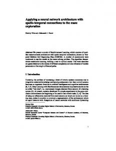
11. NETWORKSTRUCTURE The multi-sieving network is illustrated in Fig. l(a). It consists of several sieving modules connected in cascade. A sieving module may take one of two forms, i.e., RCform or R-form as shown in Fig. l(b), according to the learning task. The RC-form sieving module consists of a recognition network RN, a control network CN, an output judgement unit OJU, an AND gate, a NOT gate, and two logical switches. The R-form sieving module is similar to the RC-form, exclusive of the control network and the AND gate. Before describing each element of the sieving module, we first introduce the output coding method used in the

1319

(a). Valid output : The valid output is the correct output generated by the recognition network. That is,

recognition network.

Vjj+-xykj

‘&h’

RC-form

0:RecolplitiolrNetwork E- :Control Nelwork

0:Output Judgement Unlt (b) Figure 1: Structure of the multi-sieving neural network (a) and two forms of sieving modules (b).

A . Output Coding We focus on classification tasks as an application of neural networks. That is, the network is required to divide input data into prescribed number of sets. We use the following output coding method for the recognition network: For classification task of p 1 sets, we use p or p 1 output units. For the kth recognition network RNk, a desired output pattern ji.0 = z%,} must satisfies one of the following rules:

+

+

{zZ,zZ,...,

(c). Invalid output: Otherwise. For example, if the desired output pattern is (0, 0, l), 6 = 0.2, Z g g h = 0.8, and zEw = 0.2, then, (0.1,0.1, 0.9) is a valid output, (0.9, 0.1, 0.1) and (0.1, 0.1, 0.1) are two pseudo valid outputs, and (0.9, 0.1, 0.9) is a invalid output.

B. Output Control In order to differentiate among valid, pseudo valid and invalid outputs, the outputs produced by the recognition network are classified and controlled by an output control circuit as drawn in dotted line in Fig. l(b). The output control circuit consists of an output judgement unit OJU, a control network CN, an AND gate, a NOT gate , and two logical switches. (a) The output judgement unit is used to differentiate the invalid output from other two kinds of outputs. OJU generates 1 or 0 according to

OOJU,k

=

{

1, if z?‘ is a valid or pseudo valid output ; 0, Otherwise

(3)

where OOJU,k is the output of OJU in the kth sieving module, A = {1,2,..., tk}, tk is the number of examples used for training the kth recognition network. where Bn: = (1, 2, -.., N k } , Nk is the number of output (b) The control network is used to differentiate the valid units in RNk, and zEw and represent the low and output from the pseudo valid output. Its output is also 1 high bounds for the outputs, respectively. For example, or 0, which is determined by three output units can only represent four valid outputs as follows: ( O , O , O ) , ( O , O , l), (O,l,O) and ( l , O , O ) . Other 1, if is a valid output; %N,k = (4) four codings, (0,1, l), (l,O, l), (1,1,0) and (1,1,l), are 0, Otherwise considered to be invalid. For a given input pattern RNk may generate three where OCN,k is the output of the control network in the kth sieving module. kinds of actual outputs:

zyk

jir,

1320

(e) The network obtained by MSL algorithm is mod(c) The logical switch works as follows: If the input is "l",then the data are blocked by it. Otherwise, the data ulized. Thus, it can be constructed and implemented easily in hardware. pass through it.

111. MULTI-SIEVING LEARNING ALGORITHM Let Ti be a set of ti training samples to be learned: ~ 1 = { ( 5 7 , $)Ifori=1,2,

e..,

ti}

(5)

80

where ji: E RNI and E RNO are the input and the desired output of the ith sample, respectively. The multi-sieving learning algorithm works as follows: Step 1: Initially, a recognition network, namely RNi, is trained on the original set 2'1. Let m = 1, and proceed to the following steps. Step 2: Compute the number of valid outputs, Nvo,m, and the number of pseudo valid outputs, Npvo,m, according to Eqs. (1) and (2), respectively. If Nvo,i = t i , i.e., all ti samples are learned by the multi-sieving network, then the training is completed. If Npvo,, > 0, i.e., if there are NpVO,,pseudo valid outputs, then, a control network, namely CN,, is trained on the set of Nvo,m Npvo,, samples, corresponding to valid or pseudo valid outputs generated by RN,. If Npvo,, = 0, i.e., if there are no pseudo valid outputs, then the control network is unnecessary.

xEl

+

Step 9: Freeze the parameters of RN, and CN, (if it exists), and construct the mth sieving module as shown in Fig. l(b). Step 4: Remove Nvo,, samples which have been successfully classified by RN, from T, and create a new set of t m + l (t,+l = tm - Nvo,,) samples T '+l, which are not classified by RN,. Let m = m 1and go back to the step 2. It should be noted that we assume that the control network CNm always learns the classification of the valid and the pseudo valid outputs successfully. The multi-sieving learning algorithm has several attractive properties such as: (a) Once a sample is learned by a sieving module, then this sample will be removed from the set of samples and never been used in the training process. As a result, the deeper the multi-sieving network is, the fewer the samples become. (b) A complex task can be decomposed into several manageable subtasks automatically, and each subtask can be learned by a sieving module. (c) By adjusting the sizes of the recognition networks and the epochs used for training them, the number of sieving modules can be controlled. (d) Various sorts of the structures of RNm and CN, and the training algorithms for them can be chosen by the user.

+

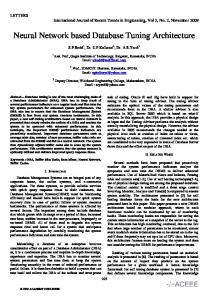
Iv. IMPLEMENTATION OF ADDITIONAL LEARNING In many applications of neural networks, the trained network may not have good generalization capability since the number of training data picked up from environments is limited. Consequently, after the training, we must examine the generalization capability of the network. If the network has poor generalization capability, we should retrain the network by adding new data. In such a case, the additional learning is required. In this section, we present an algorithm for implementing additional learning based on MSN architecture and MSL algorithm. Suppose a set of tl samples 2''' has been successfully learned by an MSN with q sieving modules, namely MSNZ,,. Now, the problem is how to add a new set of 9 1 samples U1

U1 = {(a;, a?) I f o r j = 1,2,

- - a ,

(6)

u1)

t o MSN:,,. Without loss of generality and for simplicity of illustration, we also suppose that (a) all the q sieving modules are RC-form sieving modules and (b) the numbers of the valid outputs and the pseudo valid outputs produced by the kth recognition network RN; in MSNz,, are Nvo,k and N b , k 7 respectively. Let NtoT and q : z k be the numbers o valid outputs and pseudo valid outputs generalized by the kth recognition network RNE, respectively, when the new training inputs are presented to MSN:,,. Based on MSN architecture and MSL algorithm, the additional learning can be implemented as follows: Step 1: Initially, present all u1 new training inputs to the first recognition network RNf, let m = 1, and do the following steps. Step 2: Compute N::; and N;tCm according to Eqs. (1) and (2). Step 9: If ((m 5 q)A(czl N::: = ul)),i.e., all u1 new training inputs are generalized correctly by RN! through RNQ,, then the additional learning is completed. Step 4: If ((m > q ) A (Cy=,N,",'; < ul)), then go to step 5. If ((m 5 q ) A (E==, Nt:; < ul)), then replace CNQ, with a new control network CNKw which is trained N & , N;GCm + N & , training data. on a set of If ((m 5 q)A(EglNtz? < U~)A\(N,",~W, = O)A(N,tZ, = 0)), then CNQ, remains unchanged. Let m = m 1, and go back to step 2. Step 5: Remove Cy==r Nt:: samples, which are generalized correctly by RN? through RN;, from U1 and train a new multi-sieving network, namely MSN:,, on a set of u1 N,",eY samples according to MSL algorithm. Step 6: Suppose the set of 11 E:=, N::? samples has

w:>+

+

+

- cy=,

1321

-

been successfully learned by MSNE,.

Connect MSN:,,

to

MSN~,, in series as shown in Fig. 2. Input

Valid Output

are shown in Figs. 5(a) and 5(b), respectively. The CPU time for training this network is about 160,000 seconds. Comparing the learning results shown in Figs. 4(d) and 5(b) and the CPU time, we see that the multi-sieving network is much better than MLQP. * +

Y o o

0 0 , ’ .

o +

o + oo ++

Figure 2: The connection of MSN:,,

to MSNE,,.

OO O *

o + o *

Q +

0.5. o

+

o * 0

V. SIMULATION RESULTS

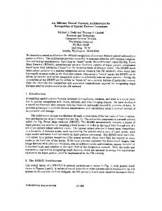
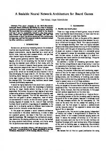
The “two-spirals” problem is chosen as a benchmark for this study because it is an extremely hard problem for BPNs [51. The training set consists of 194 (2,y) points at which the network should output 0’s or 1’s as shown in Fig. 3(d). This problem is learned by a multi-sieving network with three sieving modules. The recognition network in each sieving module has 2 input, 5 hidden and 1 output units. All the sieving modules take the R-form as shown in Fig. l(b) because there are no pseudo valid outputs in each sieving stage. In each sieving stage, the learning is stopped after 10,000 epochs if the total error is greater than a given value. Figs. 3(a) through 3(c) show the patterns that are classified by the first through the third sieving modules. The response plots of the first through the third sieving modules and the whole MSN are illustrated in Figs. 4(a) through 4(d). The CPU time for training all the recognition networks in three R-form sieving modules is about 2075 seconds on Sparc ELC workstation. This problem is also learned by a MLQP with 2 input, 40 hidden and 1 output units. The network is trained by the back-propagation algorithm. After 500,000 epochs, the network has not yet achieved the desired total error. The learning curve and the response plot of the network

“0

0”

o *

O

o + 0*+”p o o + + * * +

In this section, we will describe simulations to study the performance of MSNs in comparison with that of BPNs. The structure of RN, and CN, and the training algorithm for them are chosen to be multilayer quadratic perceptron (MLQP) [31 and the backpropagation algorithm i41, respectively. MLQP is an extension of multilayer perceptron. In MLQP, quadratic terms are introduced into the net input as well as linear terms in the conventional multilayer perceptron. It has been shown that MLQP is far superior to the conventional BPN in convergence for pattern classification problems L31. In the simulations, the learning rates are experimentally optimized in convergence speed for the specified problems with a constant coefficient (0.9) for the momentums.

A . Example 1

O +

+

o+

0 0

Y

* *

0.5.

Figure 3: Patterns classified by the first sieving module (a), the second sieving module (b), the third sieving module (c), and the whole multi-sieving network (d). For symbols “o” and “+”, the network is required to generate output 0 and 1, respectively.

B. Example 2 In this example, we will demonstrate how to implement additional learning by use of MSN architecture and MSL algorithm. A simplified version of the ‘Ltwo-spirals”problem shown in Fig. 6(a) is learned by a single recognition network RN1. The response plot of RNl is illustrated in Fig. 7(a). Now, we add 16 new samples as shown in Fig. 6(b). We construct a MSN by adding another sieving module as shown in Fig. 8 to learn the augmented problem. The role of CN1 is to differentiate the 16 new samples from the original samples. RN2 is used to recognize the 16 new samples. After the 16 new samples are learned by RN2, the response plot of the whole MSN is illustrated in Fig. 7(d). Figures 7(b) and 7(c) show the response plots of CN1 and RN2, respectively. From Figs. 7(a) and 7(d), we see that the 16 new samples have been added to the network without destroying any parameters of RN1.

1322

Figure 4: Response plots of the first sieving module (a), the second sieving module (b), the third sieving module (c), and the whole multi-sieving network (d). Black and white represent output of “0” and “l”,respectively, and grey represents intermediate value.

0.0.

0

45.

0

(4

CRI Tms=-)

(b)

After 500,000 epochs of training, the total error is still about 3.21. The learning curve is illustrated in Fig. 9(a). From this figure, it seems that the network may be trapped in a local minima, and the network can not converge to the desired error, which is set t o 0.01 in this simulation, without changing the initial parameters or network size. Examining 528 training data, we see that only 6 data are not correctly classified by RN1, and other 522 data have been successfully learned. There are no pseudo valid outputs formed in this case. In order to overcome the local minima and achieve the desired total error, we construct MSN by adding a sieving module to RBI.The first sieving module is chosen to be R-form since Nvo,l = 0. A recognition network with 10 input, 3 hidden, and 11 output units, namely R N 2 , is selected to learn the remaining 6 data which are not classified by RN1. The learning curve is shown in Fig. 9(b). From this figure, we see that R N 2 converges to the desired error quickly. After the training, the network obtained by the MSL algorithm is a MSN with two R-form sieving modules. Examining the generalization capability of RN1 amd MSN with two sieving modules on 462 test data, we obtain 38.74% correct rate for RNI, and 41.13% for MSN’. From the above results, we see that the MSN architecture can overcome local minima efficiently and the generalization capability is improved slightly after the local minima is overcome.

(4 (b) Figure 6: The original 82 samples (a) and the 16 new samples (b).

IV. CONCLUSION

Figure 5: The learning curve (a) and the response plot of MLQP for the “two-spirals” problem (b).

In this paper, a new neural network architecture MSN and a learning algorithm MSL for it are proposed. MSN architecture has several advantages over BPNs. The most imC. Exam.ple 3 portant advantages are automatic decomposition of learnThis example demonstrates how to overcome the prob- ing tasks and easy implementation of additional learning. lem of local minima by use of MSN architecture. We per- The simulation results show that MSN architecture overform simulation with a speaker independent vowel recog- comes the difficulties of local minima and slow convernition problem [6]. The vowel data consisting of 528 train- gence, which are encountered in BPNs, by decomposing ing data and 462 test data are taken from CMU learning learning tasks automatically. benchmark database 171. Initially, a single recognition network with 10 input, 11 ‘For this test data, it is difficult t o obtain a high correct rate. hidden, and 11 output units, namely RNI, is trained on R ~ b i n s o n ~has ~ ] reported that a correct rate about 44% is obtained a set of 528 samples by the backpropagation algorithm [41. by a multilayer perceptron with 11 hidden units.

1323

Furtlier refinement of MSN architecture with large pattern classification application is a subject to be studied in the future work.

Figure 9: The learning curves of RN1 (a) and RN2 (b).

(21 BaRers, P. T. and Zelle, J. M. : “Growing layers of perceptrons: Introducing the extentron algorithm”, Proc. of International Joint Conference on Neural Networks, pp. 11-392-11-397, Baltimore, MD, 1992.

[3] Lu, B. L., Bai, Y., Kita, H. and Nishikawa, Y. : “An Efficient multilayer quadratic perceptron for pattern classification and function approximation”, Proc. of the International Joint Conference on Neural Networks’93, vol. 11, pp. 1385-1388,Nagoya, 1993. [4] Oogen, A. V. and Nienhuis, B. : “Improving the convergence of the backpropagation algorithm”, Neural

Networks, vol. 5, pp. 465-471,1992. Figure 7: Response plots of RN1 (a), CN1 (b), RN2 (c), [5] Lang, K. and Witbrock, M. : “Learning to tell two and MSN (d). spirals apart”, Proc. of 1988 Connectionist Modekr Summer School, Morgan Kanfann, pp. 52-59,1988.

[6]Robinson, A. J. : “Dynamic error propagation networks”, Cambridge University, PhD. Thesis, 1989.

[7]White, M.: ”CMU learning benchmark database”, Canzegie Mellon University, School of Computer Science, 1993.

Figure 8: MSN for implementing the additional learning.

REFERENCES [l] Fahlman, S. and Lebiere, C. : “The cascade-correlation learning architecture”, Carnegie-Mellon University Report CMU-CS-90-100, 1990.

1324