Methods for Fault Detection, Diagnostics, and ... - Semantic Scholar

Copyright 2005, American Society of Heating, Refrigerating and Air-Conditioning Engineers, Inc. (www.ashrae.org). Reprinted by permission from International Journal of HVAC&R Research, Vol. 11, No. 1, January 2005. This article may not be copied nor distributed in either paper or digital form without ASHRAE’s permission.

VOLUME 11, NUMBER 1

HVAC&R RESEARCH

JANUARY 2005

REVIEW ARTICLE

Methods for Fault Detection, Diagnostics, and Prognostics for Building Systems— A Review, Part I Srinivas Katipamula, PhD

Michael R. Brambley, PhD

Member ASHRAE

Member AHSRAE

Received December 23, 2003; accepted July 20, 2004 Part II of this article will be published in Volume 11, Number 2, April 2005.

Poorly maintained, degraded, and improperly controlled equipment wastes an estimated 15% to 30% of energy used in commercial buildings. Much of this waste could be prevented with widespread adoption of automated condition-based maintenance. Automated fault detection and diagnostics (FDD) along with prognostics provide a cornerstone for condition-based maintenance of engineered systems. Although FDD has been an active area of research in other fields for more than a decade, applications for heating, ventilating, air conditioning, and refrigeration (HVAC&R) and other building systems have lagged those in other industries. Nonetheless, over the last decade there has been considerable research and development targeted toward developing FDD methods for HVAC&R equipment. Despite this research, there are still only a handful of FDD tools that are deployed in the field. This paper is the first of a two-part review of methods for automated FDD and prognostics whose intent is to increase awareness of the HVAC&R research and development community to the body of FDD and prognostics developments in other fields as well as advancements in the field of HVAC&R. This first part of the review focuses on generic FDD and prognostics, providing a framework for categorizing methods, describing them, and identifying their primary strengths and weaknesses. The second paper in this review, to be published in the April 2005 International Journal of HVAC&R Research, will address research and applications specific to the fields of HVAC&R.

INTRODUCTION FDD is an area of investigation concerned with automating the processes of detecting faults with physical systems and diagnosing their causes. Prognostics address the use of automated methods to detect and diagnose degradation of physical system performance, anticipate future failures, and project the remaining life of physical systems in acceptable operating state before faults or unacceptable degradations of performance occur. Together these methods provide a cornerstone for condition-based maintenance of engineered systems. For many years, FDD has been an active area of research and development in the aerospace, process controls, automotive, manufacturing, nuclear, and national defense fields and continues to be today. Over the last decade or so, efforts have been undertaken to bring automated fault detection, diagnosis, and prognosis to the HVAC&R field. While FDD is well established in other industries, it is still in its infancy in HVAC&R. Much of the research and development in Srinivas Katipamula is a senior research scientist and Michael R. Brambley is a staff scientist at Pacific Northwest National Laboratory, Richland, Washington.

3

4

HVAC&R RESEARCH

Figure 1. Generic application of fault detection and diagnostics to operation and maintenance of engineered systems. HVAC&R is still performed in universities and national laboratories, and commercial tools using these techniques are only beginning to emerge in this field, while in other fields such as automobiles, automated FDD has been incorporated in products for more than a decade. This paper, which is the first of two parts, provides an overview of fault detection, diagnostics, and prognostics (FDD&P) starting with descriptions of the fundamental processes and some important definitions and then identifying the strengths and weaknesses of methods across the broad spectrum of approaches. The second part will review FDD&P research in the HVAC&R field and conclude with discussion of the current state of applications in buildings and likely contributions to operating and maintaining buildings in the future (to be published in the April 2005 issue of the International Journal of HVAC&R Research).

Generic FDD Process In this section, the use of FDD in support of the operation and maintenance of engineered systems is described along with some details of the FDD process itself. The process applies to essentially all engineered systems and has been widely used to describe FDD for both critical and noncritical systems in many fields (Isermann 1984). The primary objective of an FDD system is early detection of faults and diagnosis of their causes, enabling correction of the faults before additional damage to the system or loss of service occurs. This is accomplished by continuously monitoring the operations of a system, using FDD to detect and diagnose abnormal conditions and the faults associated with them, then evaluating the significance of the detected faults, and deciding how to respond. A typical operation and maintenance process using automated FDD can be viewed as having four distinct functional processes, as shown in Figure 1; similar process descriptions have been provided by Issermann

VOLUME 11, NUMBER 1, JANUARY 2005

5

(1984) and Rossi and Braun (1997). The first step is to monitor the physical system or device and detect any abnormal conditions (problems). This step is generally referred to as fault detection. When an abnormal condition is detected, fault diagnosis is used to evaluate the fault and determine its causes. These two steps constitute the FDD process. Following diagnosis, fault evaluation assesses the size and significance of the impact on system performance (in terms of energy use, cost, availability, or effects on other performance indicators). Based on the fault evaluation, a decision is then made on how to respond to the fault (e.g., by taking a corrective action or possibly even no action). Together these four steps enable condition-based maintenance, which is referred to as an automated FDD system in this paper. In most cases, detection of faults is relatively easier than diagnosing the cause of the fault or evaluating the impacts arising from the fault. FDD itself is frequently described as consisting of three key processes: fault detection, fault isolation, and fault identification. The first, fault detection, is the process of determining that some fault has occurred in the system. The second involves isolating the specific fault that occurred, including determining the kind of fault, the location of the fault, and the time of detection. The third process, fault identification, includes determining the size and time-variant behavior of a fault. Together, fault isolation and fault identification are commonly termed fault diagnosis. Review of the literature reveals a wide array of approaches used to detect and diagnose faults. The sequencing of the detection and diagnosis varies. In some cases, the detection system runs continuously, while the diagnostic system is triggered only upon the detection of a fault. In other applications, the detection and diagnostic systems run in parallel, and in some instances, the detection and diagnostics are performed in a single step. Review of literature also indicates that most research and development in this field focuses on methods for FDD itself rather than on decision processes and tools. Approaches to FDD range from methods based on physical and analytical models to those driven by performance data and using artificial intelligence or statistical techniques. Little has been published on the fault evaluation and decision stages of the overall process in which FDD is used.

Prognostics Prognostics focus on predicting the condition of an engineered system or equipment at times in the future. As with FDD, prognostics are used along with evaluations of impacts to make operation and maintenance decisions. Use of prognostics enables transition from maintenance based on current conditions of engineered systems and equipment (condition-based maintenance) to predictive maintenance. Predictive maintenance is based on anticipated future conditions of the equipment, its remaining time before failure (or time before reaching an unacceptable level of performance), the rate of degradation, and the nature of the failure if it were to occur. Prognosis generally uses some figure of merit (FOM) to quantify the “degree of fault.” Predicting the future state and its acceptability requires three factors: (1) a measure of the system’s current FOM, (2) a model of the progression of faults, and (3) the value of the FOM at which the system fails (i.e., a fault occurs) or reaches an unacceptably poor level of performance (Greitzer and Pawlowski 2002). The current value of the FOM at any time can be determined from sensor measurements and FDD methods. The lowest value of the FOM that is acceptable is based on judgment or a mapping from FOM to failures. The model for progression of faults can be based on a theory of fault progression, on empirical data, or a combination of both. The key difference between FDD and prognostics is the need to model fault progression. Fault progression is very application-specific, and much of the work in this field is documented in the literature of the various application areas. This aspect of prognostics will not be reviewed further in this paper, which will instead focus on FDD, which, in addition to providing a basis itself for condi-

6

HVAC&R RESEARCH

Table 1. List of Survey Papers in Other Industries Author Isermann (1984) Gertler (1988a) Frank (1990) Isermann and Ballé (1997) Frank (1997)

Topic Various modeling and estimation methods for FDD Survey of model-based FDD in complex plants Survey of FDD methods based on analytical and knowledge-based redundancy for dynamic systems Trends in applications for model-based FDD New developments using artificial intelligence in fault diagnosis

tion-based operation and maintenance, also provides valuable tools for the first step of prognostics, the process of evaluating the current state of the engineered system. Although potentially important to move building maintenance from being reactive and preventive into the realm of condition-based maintenance, no research and development specifically targeted at developing and applying prognostics to building equipment is reported in the literature. Prognostics could be used to better guide the scheduling of overhauls of boilers, predict and plan for failures of pumps, fans, and the motors that drive them, time the replacement of filters and cleaning of heat exchangers (heating and cooling coils), as well as other maintenance activities. By accounting for measured rates of degradation using prognostic techniques, maintenance could be performed based on the actual condition of equipment as it compares to an acceptable range for operation rather than on preventive maintenance schedules based on industry averages and manufacturer recommendations that must include factors of safety (or, worse yet, by running until complete failure). By employing prognostics, maintenance can be timed optimally rather than be performed too soon (which is less than economically optimal) or too late (which causes disruption of operations as well as additional repair costs).

Summary of Fundamental FDD Research Several survey papers over the last three decades have summarized much of the research into the fundamental processes of automated FDD. This research grew out of needs in the fields of aeronautics, space exploration, nuclear energy, process industries, manufacturing, and national defense. The first major survey was written by Willsky (1976). Other key survey papers are identified in Table 1. The developments in fault-detection methods up to the respective times are also summarized in the books by Himmelblau (1978), Pau (1981), Patton et al. (1989), Mangoubi (1998), Gertler (1998b), Chen and Patton (1999), and Patton et al. (2003). More recently, Venkatasubramanian et al. (2003a, 2003b, 2003c) published a three-part series reviewing process fault detection and diagnosis.

FDD Research for HVAC&R Systems Unlike research on FDD in the nuclear, aerospace, process control, and national defense fields, which began decades ago, FDD research for HVAC&R systems did not begin until the late 1980s and early 1990s (Braun 1999). In the late 1980s, McKellar (1987) and Stallard (1989) explored automated FDD for vapor-compression-based refrigeration. In the 1990s, several FDD applications for building systems were developed and tested in laboratories. Most of these investigations focused on FDD for vapor compression equipment (refrigerators, air conditioners, heat pumps, and chillers) closely followed by applications to air-handling units (AHUs). In general, these applications of FDD used measured temperature and/or pressure at various locations in a system and thermodynamic relationships to detect and diagnose common faults. In the early 1990s, the International Energy Agency (IEA) commissioned the Annex 25 collaborative research project on real-time simulation of HVAC&R systems for building optimiza-


7

tion, fault detection, and diagnostics (Hyvärinen and Kärki 1996). The Annex 25 study identified common faults for various types of HVAC&R systems, and a wide variety of detection and diagnosis methods were investigated. This was followed by another IEA study to demonstrate FDD systems in real buildings (Dexter and Pakanen 2001). In the mid 1990s, the U.S. Department for Energy (DOE) funded development of a whole-building diagnostic tool, which had two diagnostic modules, one for detecting anomalies in whole-building and major system energy consumption and the other focused on FDD for outdoor-air ventilation and economizing (Brambley et al. 1998; Katipamula et al. 1999, 2003). Other DOE-funded activities include the work of Salsbury and Diamond (2001), who developed a simplified physical-model-based FDD for air-handling units, and the investigation by Sreedharan and Haves (2001), who compared three chiller models for their ability to reproduce the observed performance of a centrifugal chiller for FDD application. Also in the mid to late 1990s, a newly formed ASHRAE Technical Committee on Smart Building Systems became active in FDD research, sponsoring several research projects (Norford et al. 2002; Comstock et al. 1999, 2001; Reddy and Andersen 2002; Reddy et al. 2003). Also around the same time, the California Energy Commission through the public interest energy research (PIER) program funded projects that built on some of the previous FDD work in the HVAC&R field (AEC 2003). These commission-funded projects were completed in 2003.

Applications for FDD and Prognostics in Buildings Automated FDD and prognostics show promise in three basic areas of building engineering: (1) commissioning, (2) operation, and (3) maintenance. Commissioning involves in part ensuring that systems are installed correctly and operate properly. Problems found during commissioning include installation errors (e.g., fans installed backward), incorrectly sized equipment, and improperly implemented controls (e.g., incorrect schedules, setpoints, and algorithms) to name a few. Most of the commissioning actions that discover these problems, which include visual inspections and functional testing, are performed manually. Data might be collected during some tests using automated data loggers and analysis might be done with computers, but the process of interpreting the data and evaluating results is performed manually. FDD methods with all the capabilities shown in Figure 1 could automate much of the functional testing and interpretation of test results, ensuring completeness of testing, consistency in methods, records of all data and processing, and the ability to continuously or periodically repeat the tests throughout the life of the facility (PECI and Battelle 2003; Katipamula et al. 2002). FDD methods for application during initial building commissioning might differ from those applied later in the building’s lifetime. At start-up, no historical data are available, whereas later in the lifetime, data from earlier operation can be used in FDD. Selection of methods must consider these differences; however, automated functional testing is likely to involve short-term data collection, whether performed during initial building commissioning or during routine operation later in the building’s lifetime, and, therefore, the same methods can be used regardless of when the functional tests are performed. Such a short time period is generally required for functional testing that it obviates the possibility that the system undergoing testing may change (e.g., performance deteriorate) during the test itself. Besides use in functional testing, FDD methods could be used to test for the proper installation of equipment without requiring visual inspection. Use of labor might be minimized by only performing visual inspections to confirm installation problems after they have been detected automatically. Methods for automatically detecting and diagnosing physical configurations have not yet been developed. During building operation, FDD tools could detect and diagnose performance degradation and faults, many of which go undetected for weeks or months in most commercial buildings. Many building performance problems are compensated with automatic compensation by con-

8

HVAC&R RESEARCH

trollers so occupants experience no discomfort, but the penalty is often increased energy consumption and operating costs. Automated FDD tools could detect these as well as more obvious problems. In contrast to the short time periods over which FDD might be applied for functional testing, the time periods considered for passive fault detection during routine operation are likely much longer. Changes in the system can occur over these longer periods, but for passive FDD these changes can be used to identify operational problems, whereas during functional testing, such changes are undesirable but minimized by using short-term testing. Automated FDD tools not only detect faults and alert building operation staff to them but also identify causes of those problems so that maintenance efforts can be targeted, ultimately lowering maintenance costs and ensuring good operation. When coupled with knowledge bases on maintenance procedures, tools of the future may provide guidance on actions to correct the problems identified by FDD tools. By detecting performance degradation rather than just complete failure of a physical component, FDD tools could also help prevent catastrophic failure of systems by alerting building operation and maintenance staff to impending failures before actual failure occurs. This would enable convenient scheduling of maintenance, reduced down time from unexpected faults, and more efficient use of maintenance staff time through use of condition-based maintenance. Application of prognostics to building systems and equipment would further refine condition-based maintenance by adding predictive capabilities to the operation and maintenance tool set. Tools based on prognostics would enable predictive condition-based maintenance, further improving the basis for maintenance decisions.

Terminology Until the early 1990s most research and development in FDD was limited to nuclear power plants, aircraft, process plants, the automobile industry, and national defense. A survey of the FDD literature indicates a lack of consistent terminology. Isermann and Ballé (1997) provide a good working set of definitions from which Katipamula et al. (2001) developed a set of terms relevant to HVAC&R. The terms used in this paper conform to the definitions in Katipamula et al. (2001).

FUNDAMENTAL FDD METHODS The basic building blocks of FDD systems are the methods for detecting faults and subsequently diagnosing their causes. Several different methods are used to detect and diagnose faults. The major difference in these approaches is the knowledge used for formulating the diagnostics. At the limits, diagnostics can be based on a priori knowledge (e.g., models based entirely on first principles) or driven completely empirically (e.g., by black-box models). Both approaches use models and both use data, but the approach to formulating the diagnostics differs fundamentally. First-principle model-based approaches use a priori knowledge to specify a model that serves as the basis for identifying and evaluating differences (residuals) between the actual operating states determined from measurements and the expected operating state and values of characteristics obtained from the model. Purely process data-driven approaches (i.e., methods based on black-box models) use no a priori knowledge of the process but, instead, derive behavioral models only from measurement data from the process itself. In this latter case, the models may not have any direct physical significance. Model-based methods can use quantitative or qualitative models. Quantitative models are sets of quantitative mathematical relationships based on the underlying physics of the processes. Qualitative models are models consisting of qualitative relationships derived from knowledge of the underlying physics. The boundary between quantitative models and qualitative models can become blurred for some approaches, but this distinction and that between model-based and pro-


9

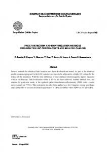
Figure 2. Classification scheme for FDD methods.

cess history (data) based methods provide a useful scheme for categorizing FDD methods, which is used in this paper (see Figure 2). Quantitative model-based methods include those based on detailed physical models as well as those based on simplified models of the physical processes. These models can be steady-state, linear dynamic, or nonlinear dynamic. Qualitative model-based approaches include rule-based systems and models based on qualitative physics. For rule-based systems, we further distinguish between those based on expert rules (i.e., expert systems) for which there may, in some cases, be no underlying first principles from physics, rules derived from first principles, and simple limit checks (which serve as the basis for alarms). In contrast to the first two groups where a priori knowledge of the process is assumed, the third group is based solely on process history, i.e., a large amount of historical data is assumed to be available. These models include black-box (input-output) methods for which the models are derived purely from the data and gray-box models that use first principles or engineering knowledge to specify the mathematical form of terms in the model but for which parameters (such as coefficients in the model) are determined from process data. Black-box methods include statistically derived models (e.g., regression), artificial neural networks (ANNs), and other pattern-recognition techniques. The broad classifications selected for this review are loosely based on the classification scheme employed by Venkatasubramanian et al. (2003a, 2003b, 2003c). Although not perfect, it provides a useful basis for contrasting basic approaches to FDD based on the nature of the knowledge used for their formulation. Key objectives for the discussion that follows are to describe each of the basic modeling techniques, to identify any constraints that would limit the application of each technique, and to assess strengths and weaknesses of each technique for application to fault detection and diagnostics. In addition, published research that uses the techniques is identified.

Quantitative Model-Based Methods This section reviews the quantitative model-based FDD methods. As the complexity of control systems and use of computers increased, quantitative model-based FDD systems became more prominent. Model-based methods rely on analytical redundancy by using explicit mathematical models of the monitored process, plant, or system to detect and diagnose faults. In contrast to physical redundancy (wherein measurements from multiple sensors are compared to

10

HVAC&R RESEARCH

each other) with analytical redundancy, sensor measurements are compared to values computed analytically, with other measured variables serving as model inputs (Gertler 1998b). Quantitative model-based approaches can be further subdivided into detailed and simplified physical models. As the name implies, physical models are based on an a priori fundamental understanding of the physical principles governing the behavior of the system. In a physical model-based FDD approach, the behavior of the system and values of outputs are modeled (predicted or estimated) for a given set of measured inputs (e.g., temperature, pressure, flow rate) and model parameters (e.g., heat transfer coefficient, number of fins, type of refrigerant) and compared to measured performance or output. The detailed physical models are based on detailed knowledge of the physical relationships and characteristics of all components in a system. Using this detailed knowledge for mechanical systems, a set of detailed mathematical equations based on mass, momentum, and energy balances along with heat and mass transfer relations are developed and solved. Detailed models can simulate both normal and “faulty” operational states of the system (although modeling of faulty states is not required by all methods). Quantitative models also have an advantage in modeling the transient behavior of the systems more precisely than any other modeling technique. Dynamic physical models are particularly important for capturing faults during transient operation. Bendapudi and Braun (2002) provide a detailed list of available dynamic models for vapor compression equipment. They also developed a dynamic centrifugal chiller model from first principles for FDD. They cautioned, however, that the model was validated only for a single chiller with specific information from the chiller manufacturer. The model can be used with other chillers, but it would require the addition of appropriate controller, compressor, and valve behavior. With the exception of the model developed by Bendapudi and Braun (2002), which was explicitly developed for FDD, most other vapor compression models have not been used as a basis for FDD. The main reason is that the level to which detailed physical characteristics must be specified for the system and subsystems is not always easy to obtain and apply, and the application of the method in near real-time is computationally intensive. For example, to truly model the transient phenomena in a heat exchanger of a vapor compression system, it is necessary to create a detailed inventory of the mass distribution at all points in the heat exchanger as a function of time, requiring solution of the Navier-Stokes equations for compressible flow (Bendapudi and Braun 2002). As part of ASHRAE Research Project 738, Lebrun and Bourdouxhe (1996) reviewed dynamic HVAC models. This research identified and described the available dynamic models for HVAC-related equipment from over 500 references that cover duct and pipe models, heat and mass exchanger models, models of airflow dynamics, boiler and furnace models, heat pump and chiller models (including vapor compression and absorption systems, compressors, condensers, evaporators, expansion valves, and control), controllers, sensors, and actuators. Other research papers related to this work include Bourdouxhe et al. (1994a, 1994b, 1995, 1997). Another ASHRAE research project developed a toolkit of secondary HVAC system models (Brandemuehl and Gable 1994). In contrast to the detailed physical modeling techniques, simplified physical modeling generally employs a lumped parameter approach, which is computationally simpler because coupled space-time partial differential equations in mass, momentum, and energy balances are transformed into ordinary differential and algebraic equations. There are a number of papers that apply FDD methods based on such a modeling technique for HVAC&R systems. Although over the years a number of physical models of HVAC&R systems were developed, only a handful have actually been used in FDD implementations (Wagner and Shoureshi 1992; Haves et al. 1996; Salsbury and Diamond 2001; Norford et al. 2002; Castro 2002).


11

Strengths of Quantitative Models. Strengths of FDD based on quantitative models include: • Models are based on sound physical or engineering principles. • They provide the most accurate estimators of output when they are well formulated. • Detailed models based on first principles can model both normal and “faulty” operation; therefore, “faulty” operation can be easily distinguished from normal operation. • The transients in a dynamic system can only be modeled with detailed physical models. Weakness of Quantitative Models. Weaknesses of FDD based on quantitative models include: • They can be complex and computationally intensive. • The effort required to develop a model is significant. • These models generally require many inputs to describe the system, some for which values may not be readily available. • Extensive user input creates opportunities for poor judgment or input errors that can have significant impacts on results. Suitability of Quantitative Models. FDD based on detailed physical models is unlikely to emerge as the method of choice in the near future because of the weaknesses listed above, but simplified physical models will continue to make inroads into FDD applications.

Qualitative Model-Based Methods Fault detection and diagnostics based on qualitative modeling techniques represent another broad category that is based on a priori knowledge of the system. Unlike quantitative modeling techniques in which knowledge of the system is expressed in terms of quantitative mathematical relationships, qualitative models use qualitative relationships or knowledge bases to draw conclusions regarding the state of a system and its components (e.g., whether operations are “faulty” or “normal”). Some qualitative models are obtained by deriving knowledge statements from process history data (such as for expert systems where human experience with a process is used to derive rules governing proper and faulty operation). Qualitative model-based methods can be further subdivided into rule-based and qualitative physics-based models (see Figure 2). Both these qualitative modeling techniques employ causal knowledge of the process or system to diagnose faults. Other qualitative causal models include bond graphs (Ghiaus 1999) and case-based reasoning (Dexter and Pakenen 2001). Qualitative models can also be based on abstraction hierarchies based on decomposition (Venkatasubramanian 2003b), which is the ability to draw inferences about the behavior of the overall system solely from the laws governing the behavior of its subsystems. More details on abstraction hierarchies and their application to problems in the process industry can be found in Venkatasubramanian (2003b). Commonly used measurement techniques provide quantitative output (e.g., temperatures, pressures, and humidities). Some qualitative methods accept quantitative inputs directly, but others require qualitative inputs (e.g., linguistic statements) so that preprocessing is required before quantitative data are used. Fuzzy logic provides a mechanism for converting such quantitative data to qualitative information. A commonly used example is the conversion of air temperature measurements to qualitative categories of hot, warm, comfortable, cool, and cold. The boundaries between these qualitative categories are “fuzzy” and fuzzy logic provides a mechanism for conversion. The outputs of “fuzzification” can then be used as inputs to qualitative diagnostic processes.

Rule-Based Systems The rule-based modeling techniques use a priori knowledge to derive a set of if-then-else rules and an inference mechanism that searches through the rule-space to draw conclusions.

12

HVAC&R RESEARCH

Rule-based systems can be based solely on expert knowledge (which is inferred from experience) or can be based on first principles. We are also including FDD methods that use simple limits (to trigger alarms) in this category because they can be viewed as a limiting case of rule-based systems. Expert systems are computer-based applications used to deploy the insights, knowledge, and/or guidance of individuals with expertise in a given field. In developing expert systems, the knowledge of domain experts is usually elicited through interviews with a knowledge engineer, who later enters the collected information into a database (often referred to as a knowledge base) in the form of if-then-else statements. Some expert systems enable users to enter confidence levels along with the information for which the user is uncertain. It can also be based on practically derived rules or approximations that have been tested and proved to be operationally useful (PECI and Battelle 2003). Expert systems are usually deployed using software packages referred to as expert system shells. An expert system shell includes a software component called an inference engine, which is capable of inferring conclusions (e.g., a diagnosis) and additional information it needs in order to reach a conclusion or diagnosis if not possible initially. Expert systems have been developed to diagnose and analyze problems in many fields. Systems for medical diagnosis are among the most widely recognized. Prototype systems have been developed to perform diagnoses for operational problems in commercial building systems. Kaler (1988, 1990) described the development of an embedded expert system for monitoring packaged HVAC equipment. Kilma (1990) describes an expert system to troubleshoot operational problems in solar hot water systems. Kaldorf and Gruber (2002) describe an expert system for FDD of building systems. There are a number of other papers that describe the use of expert and knowledge-based systems (Georgescu et al. 1993; Katipamula et al. 1999), although to our knowledge, none has been successfully commercialized or has achieved widespread acceptance. A detailed description of use of expert systems in process industries is provided by Venkatasubramanian (2003c), and Patel and Kamrani (1996) provide a table of expert systems for diagnosis and maintenance. The strengths of expert systems are ease of development, transparent reasoning, ability to reason even under uncertainty, and the ability to provide explanations for the conclusions reached (Venkatasubramanian 2003b). The main weaknesses are that they are very specific to a system, can miserably fail beyond the boundaries of the knowledge incorporated in them, and are difficult to update or change. A second category of methods under rule-based approaches uses rules derived from first principles (Brambley et al. 1998; Katipamula et al. 1999; House et al. 2001). As part of its mission in commercial buildings research and development, the U.S. Department of Energy (DOE) in collaboration with industry developed a tool that automates detection and diagnosis of problems associated with outdoor-air ventilation and economizer operation. The tool, known as the outdoor-air economizer (OAE) diagnostician, monitors the performance of AHUs and detects problems with outside-air control and economizer operation, using sensors that are commonly installed for control purposes (Brambley et al. 1998; Katipamula et al. 1999). The tool diagnoses the operating conditions of AHUs using rules derived from engineering models of proper and improper air-handler performance. These rules are implemented in a decision tree structure in software. The diagnostician uses data collected periodically (e.g., from a building automation system) to navigate the decision tree and reach conclusions regarding the operating state of the AHU. At each point in the tree, a rule is evaluated based on the data, and the result determines which branch the diagnosis follows. A conclusion is reached regarding the current condition of the AHU when the end of a branch is reached. An overview of the logic tree


13

Figure 3. Overview of the tree of OAE diagnostic rules, showing key operating states.

used to identify operational states and to build the lists of possible failures is illustrated in Figure 3. The boxes represent major subprocesses necessary to determine the operating state of the air-handler, diamonds represent tests (decisions), and ovals represent end states and contain brief descriptions of “OK” and “not OK” states. Only selected end states are shown in this overview. The implementation details are provided in PECI and Battelle (2003) and Katipamula et al. (2002). House et al. (2001) developed a set of rules referred to as APAR (AHU performance assessment rules) to detect faults in AHUs. APAR rules are derived using qualitative models, similar to the approach used by Glass et al. (1995), described later in this paper. Furthermore, these rules are also similar to the rules used by Katipamula et al. (1999). Twenty-eight rules were derived to represent faults in various operating modes of the AHU, and possible causes of the

14

HVAC&R RESEARCH

faults were identified as well. Rules were also associated with impact on comfort, indoor air quality, energy, and maintenance and/or equipment life. The process uses control signals and occupancy information to identify the operating mode of the AHU (e.g., heating, cooling, economizing), which leads to a subset of rules that specify temperature relationships that are applicable for that mode. APAR rules were written such that if a rule is satisfied, a fault is indicated or implied. The process first establishes the mode of operation; then rules based on conservation of mass and energy can be used along with the sensor information that is typically available for controlling the AHU. For example, normal operation in economizing mode with 100% outdoor air dictates that the outdoor-air and mixed-air temperatures must be approximately equal. Defining To and Tm as the outdoor and mixed-air temperatures, respectively, the rule is written as: If |To − Tm| > εt, then an economizer fault has occurred, where εt is a threshold that depends on the uncertainty (or accuracy) of the measurements. If the rule is satisfied, then it indicates a fault. The validity and robustness of the rule set was assessed through data generated from a series of simulations. After testing the rule set with simulated data, the rules were used on five AHUs in a real building. Various faults were identified with all five AHUs (stuck dampers and manual override of control signals). The authors acknowledge that selection of thresholds is critical to successful implementation and have suggested additional work in this area. Additional testing and validation for APAR was preformed by Castro et al. (2003) as part of work for the California Energy Commission. Other research papers that employ qualitative models include Glass et al. (1995) and Karki and Karjalainen (1999). Sisk et al. (2003) provide a set of data flow diagrams for diagnostics that express a set of rules for detecting faults with chillers, boilers, chilled-water distribution, and cooling towers. The rules use as inputs the status of equipment and measurements of temperature and the current drawn by various pieces of equipment, including chillers, pumps, and fans. Fault trees and directed graphs (digraphs) are two methods that can be used to generate rules from first principles knowledge (Venkatasubramanian 2003b). Cause-effect relations or models can be represented especially well in the form of signed directed graphs (SDG). Directed graphs use arcs to connect nodes (state variables), and an SDG is a graph in which the directed arcs have a positive or a negative sign attached to them. A positive sign indicates that a relationship is reinforcing, and a negative sign indicates that the relationship is suppressing. From SDG, cause-effect graphs (CE graphs) can be developed for fault diagnosis. Shiozaki and Miyasaka (1999) used SDG to represent a causality model for a variable-air-volume (VAV) AHU. Since the advent of computers in the process control industry, limit checks and alarms based on them have become commonplace (Gertler 1988a). Early deployments relied on simple limit checking for fault detection. Even the early fault detection systems for the Space Shuttles’ main engines, while on the ground, primarily used limit checking with fixed thresholds on each measured variable (Cikanek 1986). This technique is still used in data-rich environments with redundant sensors. This method relies on comparing raw outputs that are directly measured using sensors or estimated expected values of characteristic quantities calculated from available measurements with expected values. A fault is indicated if the comparison residual (actual value – expected value) exceeds a predefined threshold. The characteristic quantities are features that cannot be directly measured but can be computed from other measured quantities, for example, the outdoor-air fraction for the air-handling unit or the coefficient-of-performance of an air conditioner. Because the measured quantities are compared to fixed thresholds, applications are limited to nondynamic systems. Also, anticipating if or when a fault would occur is difficult using this approach.


15

Qualitative Physics-Based Models Qualitative models enable conclusions to be reached about the state of a system with incomplete or uncertain knowledge of the physical process (de Kleer and Brown 1984). Two basic approaches are used. The first is the derivation of qualitative confluence equations from the ordinary differential equations governing behavior of the process. These equations can then be solved using imprecise information (e.g., order of magnitude inputs), using a qualitative algebra, to derive the qualitative behavior of the system. The second approach involves deriving qualitative behaviors from the ordinary differential equations governing the physical behavior of the system. The qualitative behaviors can then be used as a source of knowledge for FDD. These methods “start from a description of the physical mechanism, construct a model, and then use an algorithm so as to determine all of the behaviors of the system without precise knowledge of the parameters and functional relationships” (Venkatasubramanian 2003b). Practical applications of qualitative physical models for FDD have been explored using qualitative simulation (Kay 1998) and by applying qualitative process theory (QPT) (see Venkatasubramanian 2003b for more details). The primary advantage of qualitative physics-based models is that they enable conclusions about a process without exact expressions governing the process and precise numerical inputs. In some cases, partial conclusions can be reached from incomplete and uncertain knowledge of the system and inputs. The authors found no examples of application of qualitative physics to FDD for HVAC&R in the literature. Strengths of Qualitative Models. Strengths of qualitative models are: • They are well suited for data-rich environments and noncritical processes. • These methods are simple to develop and apply. • Their reasoning is transparent, and they provide the ability to reason even under uncertainty. • They possess the ability to provide explanations for the suggested diagnoses because the method relies on cause-effect relationships. • Some methods provide the ability to perform FDD without precise knowledge of the system and exact numerical values for inputs and parameters. Weaknesses of Qualitative Models. Weaknesses of FDD based on qualitative models include: • The methods are specific to a system or a process. • Although these methods are easy to develop, it is difficult to ensure that all rules are always applicable and to find a complete set of rules, especially when the system is complex. • As new rules are added to extend the existing rules or accommodate special circumstances, the simplicity is lost. • These models, to a large extent, depend on the expertise and knowledge of the developer. Suitability of Qualitative Models. Qualitative methods provide shortcuts and may offer the most expedient way to meet analytical needs where more rigorous approaches are time or cost prohibitive.

FDD Methods Based on Models Derived from Process History In a process history-based (data-driven) model, both inputs and outputs are known and measured. The main objective of a data-driven model is to mathematically relate measured inputs to measured outputs. There are a number of ways the input/output data can be transformed and used as a priori knowledge in a diagnostic system. This process of transformation is also known as feature extraction or parameter extraction. When the model features or parameters have no physical significance, these models are referred to as black-box models. Some examples of black-box modeling techniques include: linear (LR) or multiple linear regression (MLR), artifi-

16

HVAC&R RESEARCH

cial neural networks (ANNs), and fuzzy logic (FL). Model parameters of an empirical model that is carefully crafted based on first principles often have physical significance; these models are referred to as gray-box or mechanistic models. Gray-box models often use linear or multiple linear regressions to estimate model parameters (e.g., coefficients) from measured inputs and outputs, while preserving the physical significance of terms appearing in the models.

Gray-Box Models In a gray-box approach, the functional form of the model is formulated in such a way that the parameter estimates can be traced to actual physical principles that govern the performance of the system being modeled. Examples of studies of parameter estimation applied to building systems include Sonderegger (1977), Subbarao (1988), Rabl (1988), Reddy (1989), Braun (1990), Gordon and Ng (2000, 1995) and Guyon and Palomo (1999). Gordon and Ng (2000) developed a model based on first principles of thermodynamics and linearized heat losses. The model predicts chiller COP (ratio of evaporator cooling capacity to compressor power consumption) as a function of three specially chosen independent parameters. These independent parameters are derived from three measured quantities: cooling load (Qch), condenser inlet water temperature (Tcdi), and chilled water inlet temperature to the evaporator (Tchi). To estimate the cooling load on the evaporator, the chilled water supply temperature and the chilled water flow rate are required. Based on these quantities, the form of the universal chiller model developed by Gordon and Ng (2000) is ( T cdi – T chi ) T chi T chi ( 1 ⁄ COP + 1 )Q ch 1 ⎛ ----------- + 1⎞ --------– 1 = a 1 --------- + a 2 ------------------------------ + a 3 ------------------------------------------- , ⎝ COP ⎠ T cdi T cdi Q ch T cdi T cdi

where the temperatures are in absolute units, and the parameters (coefficients a1, a2, and a3) of the model have physical meaning in terms of irreversibility. The physical significance of these parameters is as follows: a1 a2 a3

= ∆S, total internal entropy production rate in the chiller due to internal irreversibilities, = Qleak, rate of heat losses (or gains) from (or into) the chiller, = R total heat exchanger thermal resistances, which represents the irreversibility due to finite-rate heat exchange.

The constants, or parameters a1, a2, and a3 , are determined using linear regression applied to a set of historical training data obtained from the equipment manufacturer, from laboratory tests, or from the field when the unit is operating normally (i.e., in an “unfaulted” state). There are some advantages in using models that are based on physical reasoning as compared to the simple polynomial correlations that are typically employed. In particular, fewer data usually are required to obtain an acceptable fit, and there is better confidence that the model extrapolates well to operating conditions outside the range used to obtain the correlations. Jiang and Reddy (2003) found that the Gordon and Ng (1995) model provided an excellent fit to many different chiller types. Reddy et al. (2003) note that although Qleak is typically an order of magnitude smaller than the other two terms, it should be retained in the model if the other two parameters are used for chiller diagnostics. Jia and Reddy (2003) proposed another gray-box approach called characteristic parameter model for chillers. The characteristic parameter model actually is a set of five models, each representing one of the components or characteristics of the system, namely: (1) COP, (2) compressor, (3) condenser, (4) evaporator, and (5) expansion valve. The five models are based on first principles of thermodynamics. The advantage of this approach over that of Gordon and Ng (2000) is that it will, to some extent, diagnose potential faulty operations. It requires, however, several additional measurements beyond those required by the method of Gordon and Ng


17

(2000), which are (1) cooling load, (2) condenser inlet and outlet temperatures, (3) evaporator inlet and outlet temperatures, (4) evaporator and condenser water flows, (5) suction pressure, (6) discharge pressure, (7) suction temperature, (8) condenser refrigerant temperature, (9) condenser outlet pressure, and (10) evaporator inlet pressure. Parameter estimates from gray-box models tend to be more robust than those from black-box models, which can lead to better model predictions. In general, these models have a simple form and are, therefore, easy to use. Gray-box models have a great potential for FDD and on-line controls applications. Although these models are derived from measured data, they can be used for limited extrapolation outside the range of the training data because they are formulated from first principles. They require a high level of user expertise both in formulating the appropriate form (equation) for the model and in the estimation of model parameters. As with other data-driven methods, extensive measured data often are required. For the model estimates to be meaningful and robust, measurement errors should be minimized because small uncertainties in measured data can result in relatively large changes in the physical parameters (Reddy and Anderson 2002).

Black-Box Models Black-box models are developed in a similar manner to gray-box models, but the estimated model parameters have no physical significance. Various statistical and nonstatistical methods are used to develop the relationship between inputs and outputs. Some examples of statistical methods include linear and multiple regression, polynomial regression, principle component analysis, partial least squares, and logistic regression. Nonstatistical methods include artificial neural networks (ANNs) and other pattern-recognition methods. Black-box models often require less time and effort to develop and apply compared to gray-box approaches; however, the prediction accuracy is generally lower than for gray-box models, and they cannot be used to extrapolate beyond the data range for which they were developed. A number of researchers have used a statistical black-box approach for FDD (Norford and Little 1993; Rossi 1995; Lee et al. 1996a; Peitsman and Bakker 1996; Yoshida et al. 1996; Rossi and Braun 1997; Peitsman and Soethout 1997; Breuker 1997; Breuker and Braun 1998a; Yoshida and Kumar 1999; Kumar et al. 2001; Norford et al. 2002; Riemer et al. 2002; Reddy and Andersen 2002; Andersen and Reddy 2002; Reddy et al. 2003). Rossi and Braun (1997) and Breuker and Braun (1998b) developed and evaluated a complete FDD system for packaged air-conditioning equipment. Seven black-box steady-state models are used to describe the relationship between the driving conditions and the expected output states in a normally operating system. In a normally operating, simple packaged air-conditioning unit (with on/off compressor control and fixed-speed fans), all of the output states (Y) in the system are assumed to be functions of only three driving conditions (U) that affect the operating states of the unit: the temperature of the ambient air into the condenser coil (Tamb), the temperature of the return air into the evaporator coil (Tra), and wet-bulb temperature (Twb) of the return air entering the evaporator coil. The black-box models take the polynomial form: 2

2

2

y i = a 1 + a 2 T wb + a 3 T ra + a 4 T amb + a 5 T wb + a 6 T ra + a 7 T amb 3

3

3

+ a 8 T wb T ra + a 9 T ra T amb + a 10 T wb T amb + a 11 T wb + a 12 T ra + a 13 T amb 2

2

2

2

2

+ a 14 T wb T ra + a 15 T wb T amb + a 16 T ra T wb + a 17 T ra T amb + a 18 T amb T wb 2

+ a 19 T amb T ra + a 20 T wb T ra T amb + ……… ,

18

HVAC&R RESEARCH

where yi is the ith output variable prediction and the a’s are coefficients determined using linear regression. The polynomial is fit to steady-state training data obtained in the laboratory and compared with a separate set of steady-state test data for validation. A number of researchers also used black-box models based on ANNs for FDD (Peitsman and Bakker 1996; Lee et al. 1996b; Bailey 1998; Morisot and Marchio 1999; Zmeureanu 2002; Reddy et al. 2003). ANNs are so named because they were first proposed as a model of neurobiological processes. ANNs can be viewed as sets of interconnected nodes usually arranged in multiple layers (input, hidden, and output). The nodes of the network serve as the computational elements and pass data to the other nodes to which they are connected. Although there are a number of ways to use ANN models, the models used for FDD can be broadly classified into two groups based on network architecture (e.g., sigmoidal and radial) and learning strategy (supervised vs. unsupervised). In general, ANNs learn the functional mapping of inputs to outputs using input/output training pairs. Unlike other statistical black-box approaches, ANNs have an advantage in that they model complex functional relationships with relative ease without detailed knowledge of the physics of the system. They can model nonlinear system behavior and are highly effective at recognizing patterns. Like other black-box approaches, ANNs are not good at predicting behavior that is not present in the training set, and they require a vast amount of data to be adequately trained. Strengths of Process History-Based Models. The strengths of FDD methods based on process history are: • These methods are well suited to problems for which theoretical models of behavior are poorly developed or inadequate to explain observed performance. • They are suited where training data are plentiful or inexpensive to create or collect. • Black-box models are easy to develop and do not require an understanding of the physics of the system being modeled. • Computational requirements vary, but they are generally manageable. • There is a wealth of documented information available on the underlying mathematical methods. Weaknesses of Process History-Based Models. Weaknesses of process history-based methods of FDD include: • Gray-box models based on first principles require a thorough understanding of the system and expertise in statistics. • Most models cannot be used to extrapolate beyond the range of the training data. • A large amount of training data is needed, representing both normal and “faulty” operation. • The models are specific to the system for which they are trained and rarely can be used on other systems. Suitability of Process History-Based Models. Process history-based methods are suitable where no other methods exist. Some are applicable for virtually any kind of pattern-recognition problem.

A Note on Fuzzy Logic Although fuzzy logic is not listed as an FDD method in Figure 2 because it is not a source of knowledge, it is used in the field of FDD with many of the listed methods, particularly those that are qualitative model-based and process history-based. Fuzzy set theory can account for uncertainties associated with describing the system (Hyvärinen and Kärki 1996), describing inputs to FDD, as well as classifying FDD outputs. For details of fuzzy implementation in HVAC&R refer to Hyvärinen and Kärki (1996), Ngo and Dexter (1999), and Dexter and Ngo (2001). The main advantage of using fuzzy logic is that it can account for uncertainty and nonlinear behavior in systems. In addition, software implementation is relatively easy and computationally unde-


19

manding (Dexter and Pakanen 2001). The main disadvantage of incorporating fuzzy theory in FDD is that the results are less precise compared to other approaches (Dexter and Pakanen 2001).

SELECTION OF METHODS FOR FDD APPLICATIONS Selection of method(s) for FDD plays a critical part in the development of the FDD system. As discussed in the previous section, there is a wide range of methods available for FDD. Most of them perform more than adequately in the laboratory or test setting, but not many of them may be suitable for field implementation. Some methods have few data requirements (e.g., qualitative models), while others require extensive data (e.g., process history-based methods). This section provides a brief discussion of how to properly select a method for FDD. There are several approaches to detecting and diagnosing faults in building systems. They differ widely depending on the type of system to which they are applied, the necessary degree of knowledge about the diagnosed object, cost-to-benefit ratio (including monetary as well as life safety related issues), the degree of automation, tolerance to false alarms, and the input data required. The earliest FDD methods used alarm limits as fault criteria, whereas modern methods use thresholds and statistical criteria applied to sophisticated quantitative, qualitative, and process history-based models. Between the two groups are various simplified empirical and heuristic knowledge-based methods of fault detection and diagnostics. Development of detailed physical models is expensive and not practical in most instances. Therefore, either simplified models based on first principles or heuristic knowledge bases are widely used for FDD in the HVAC&R literature. The success of the FDD system depends on proper selection of methods for both detection and diagnosis. Often methods are selected because of the interest of the developer or the availability of an existing tool. While this approach may yield satisfactory results for small-scale laboratory applications, it often leads to problems in full-scale real-life implementations. For some FDD applications, fault diagnosis may not be needed because detection sufficiently isolates the fault. On the other hand, fault diagnosis may not be possible because of lack of resolution in the data. Selection of the best method for detection and diagnosis depends on several factors. The methods used for detection are often different from the methods used for diagnosis. During detection, actual measurements (actual state or value of a parameter derived from measurements) are compared to expected values to identify that an abnormal condition has occurred. Diagnosis is more complex and requires sophisticated search methods to isolate the fault and its cause. From a survey of the literature both in critical processes and in the HVAC&R area, simplified physical and black-box modeling approaches were found widely used in detecting faults. For diagnosis, classification methods such as ANNs, fuzzy clustering1 and rule-based reasoning methods were widely used. The amount of measured data required plays a critical role in the selection of a method for both detection and diagnosis. A limited set of measured data will lead to selection of a detailed or moderately detailed physical model for detection. However, physical models may require other inputs, such as physical characteristics and design details of the system. For diagnosis, a set of fault models and a technique for selecting the fault models for a given set of inputs and outputs may be necessary. In general, most building HVAC&R systems will have a limited set of sensors—sensors that are required for control purposes only. The cost of additional sensors should be considered when selecting methods that require data beyond those that are normally 1Fuzzy clustering refers to the use of fuzzy methods with conventional clustering techniques. Cluster analysis is a technique used to partition a data set into clusters or classes, where similar data are assigned to the same cluster while dissimilar data are assigned to different clusters. In reality there is often an overlap of boundary between clusters. Fuzzy methods are better suited when there is ambiguity and, therefore, are used in combination with clustering.

20

HVAC&R RESEARCH

provided for controls, ensuring that the additional value compensates for any increase in cost. On the other hand, methods that rely on a limited set of measured data may not be sensitive to detection and may have difficulty in isolating causes of faults. If the system is extensively instrumented, classical limit checks and simplified empirical models often are sufficient for detection, while rule-based or knowledge-based models are needed for diagnosing fault causes. Before selecting methods for detection and diagnosis, a good understanding of the anticipated faults is essential. Some faults influence the selection of a diagnostic method more than the detection. Examples of faults that make diagnosis difficult include faults that exhibit different symptoms at different times, faults that are intermittent, and multiple simultaneous faults. Not many methods can diagnose the fault that exhibits different symptoms at different times and depends on the operational dynamics of the system. For example, if an outdoor-air damper is stuck wide open and the outdoor-air condition is favorable for economizing, no fault is evident. However, if the outdoor-air condition is not favorable for economizing, the stuck damper is recognizable as a fault. In addition, multiple simultaneous faults make determining the causes of faults even more difficult. To a lesser extent, the cost of development and deployment of an FDD system can influence the methods selected. Because the building industry is highly cost sensitive and safety is not generally an issue with the building systems, the methods used for detection and diagnosis have to rely on the limited set of measured data generally available. Lower costs for sensors in the future could change this situation, allowing for the installation of more sensors in building systems. For noncritical applications (i.e., those not related to life safety or having enormous costs), the methods used for detection and diagnosis should minimize the number of false positives (false alarms). If an FDD system provides users alarms for a large number of false positive faults, the users may become frustrated, lose confidence in the system, and even disable it completely in response. This is particularly important to avoid in the early stages of introducing a new technology. As a result, FDD methods applied to noncritical systems (e.g., most building systems) should be tuned to generate fewer false alarms. In contrast, FDD methods applied to critical systems must be tuned to be very sensitive to fault detection so as not to miss any instances of faults; therefore, these applications are highly sensitive and more prone to generating false alarms.

CONCLUSIONS In the first part of this two-part review, we have provided a classification scheme for FDD methods and have identified the strengths and weakness of each approach. The FDD methods were classified into three main groups: (1) quantitative model-based methods, (2) qualitative model-based methods, and (3) methods based on process history. Although quantitative model-based FDD methods are most accurate and reliable, they are generally more complex and computationally intensive compared to models based on other approaches. Therefore, these are unlikely to be the methods of choice in the near future, especially for real-time applications. The second group of FDD methods uses qualitative relationships or knowledge bases to draw conclusions regarding the state of a system. These methods are well suited for data-rich environments and noncritical processes. Because these methods provide shortcuts, they may represent the most expedient way to meet analytical needs where more processing-intensive approaches are time and cost prohibitive. The last group of methods uses historical data from processes to develop models. These models are easy to develop and use and, therefore, suitable for virtually any kind of problem for which significant amounts of measured data are available.


21

ACKNOWLEDGMENTS The review presented in this paper was funded partially by the Office of Building Technology Programs in the Office of Energy Efficiency and Renewable Energy of the U.S Department of Energy as part of the Building Systems Program at Pacific Northwest National Laboratory. The Laboratory is operated for the U.S. Department of Energy by Battelle Memorial Institute under contract DE-AC06-76RLO 1830.

REFERENCES Andersen, K.K., and T.A. Reddy, 2002. The error in variables (EIV) regression approach as a means of identifying unbiased physical parameter estimates: Application to chiller performance data. International Journal of Heating, Ventilating, Air Conditioning and Refrigerating Research 8(3):295-309. AEC (Architectural Energy Corporation). 2003. Final Report: Energy efficient and affordable commercial and residential buildings. Report prepared for the California Energy Commission. Report number P500-03-096, Architectural Energy Corporation, Boulder, Colorado. Available on the Web at http://www.archenergy.com/cec-eeb/P500-03-096-rev2-final.pdf. Bailey, M.B. 1998. The design and viability of a probabilistic fault detection and diagnosis method for vapor compression cycle equipment. Ph.D. thesis, School of Civil Engineering of University of Colorado, Boulder, Colorado. Bendapudi S., and J.E. Braun. 2002. A review of literature on dynamic models for vapor compression equipment. HL 2002-9, Report #4036-5, Ray Herrick Laboratories, Purdue University. Bourdouxhe, J.P., M. Grodent, J. Lebrun, and C. Saavedra. 1994a. A toolkit for primary HVAC system energy calculation—Part 1: Boiler model. ASHRAE Transactions 100(2):759-73. Bourdouxhe, J.P., M. Grodent, J. Lebrun, C. Saavedra, and K. Silva. 1994b. A toolkit for primary HVAC system energy calculation—Part 2: Reciprocating chiller models. ASHRAE Transactions 100(2):774-86. Bourdouxhe, J.P., M. Grodent, and C. Silva. 1995. Cooling tower model developed in a toolkit for primary HVAC system energy calculation—Part 1: Model description and validation using catalog data. Proceedings Fourth International Conference on System Simulation in Buildings. IBPSA Building Simulation '95, Madison, Wisconsin, August 14-16, 1995. Bourdouxhe, J.P., M. Grodent, and J. Lebrun. 1997. HVAC1 Toolkit: Algorithms and Subroutines for Primary HVAC Systems Energy Calculations. Atlanta: American Society Heating Refrigeration Air Conditioning Engineers, Inc. Brambley, M.R., R.G. Pratt, D.P. Chassin, and S. Katipamula. 1998. Automated diagnostics for outdoor air ventilation and economizers. ASHRAE Journal 40(10):49-55 [October]. Brandemuehl, M.J., and S. Gabel. 1994. Development of a toolkit for secondary HVAC system energy calculations. ASHRAE Transactions 100(1):21-32. Braun, J.E. 1990. Reducing energy costs and peak electrical demand through optimal control of building thermal mass. ASHRAE Transactions 96(2):876-88. Braun, J.E. 1999. Automated fault detection and diagnostics for the HVAC&R industry. International Journal of Heating, Ventilating, Air Conditioning and Refrigerating Research 5(2):85-86. Breuker, M.S. 1997. Evaluation of a statistical, rule-based fault detection and diagnostics method for vapor compression air conditioners. Master's thesis, School of Mechanical Engineering, Purdue University, West Lafayette, Indiana. Breuker, M.S., and J.E. Braun. 1998a. Common faults and their impacts for rooftop air conditioners. International Journal of Heating, Ventilating, Air Conditioning and Refrigerating Research 4(3):303-318. Breuker, M.S., and J.E. Braun. 1998b. Evaluating the performance of a fault detection and diagnostic system for vapor compression equipment. International Journal of Heating, Ventilating, Air Conditioning and Refrigerating Research 4(4):401-425. Castro, N.S., J. Schein, C. Park, M.A. Galler, S.T. Bushby, and J. M. House. 2003. Results from simulation and laboratory testing of air handling unit and variable air volume box diagnostic tools. National Institute of Standards and Technology, Gaithersburg, MD, NISTIR 6964.

22

HVAC&R RESEARCH

Castro, N. 2002. Performance evaluation of a reciprocating chiller using experimental data and model predictions for fault detection and diagnosis. ASHRAE Transactions 108(1). Chen, J., and R.J. Patton. 1999. Robust Model-Based Fault-Diagnosis for Dynamic Systems. Norwell, Massachusetts: Kluwer Academic Publishers. Cikanek, H.A., III. 1986. Space Shuttle main engine failure detection. IEEE Control Systems Magazine 6(3):13-18. Comstock, M.C., B. Chen, and J.E. Braun. 1999. Literature review for application of fault detection and diagnostic methods to vapor compression cooling equipment. HL 1999-19, Report #4036-2, Ray Herrick Laboratories, Purdue University. Comstock, M.C., J.E. Braun, and E.A. Groll. 2001. The sensitivity of chiller performance to common faults. International Journal of Heating, Ventilating, Air Conditioning and Refrigerating Research 7(3). de Kleer, J., and J.S. Brown. 1984. A qualitative physics based on sonfluence. Artificial Intelligence 24:7-83. Dexter, A., and J. Pakanen (eds.). 2001. International Energy Agency Building Demonstrating Automated Fault Detection and Diagnosis Methods in Real Buildings. Technical Research Centre of Finland, Laboratory of Heating and Ventilation, Espoo, Finland. Dexter, A.L., and D. Ngo. 2001. Fault diagnosis in air-conditioning systems: A multi-step fuzzy model-based approach. International Journal of Heating, Ventilating, Air Conditioning and Refrigerating Research 7(1):83-102. Frank, P.M. 1990. Fault diagnosis in dynamic systems using analytical and knowledge-based redundancy–A survey and some new results. Automatica 26:459-474. Frank, P.M. 1997. New developments using AI in fault diagnosis. Engng. Applic. Artif. Intell. 10(1):3-14. Georgescu, C., A. Afshari, and G. Bornard. 1993. A model-based adaptive predictor fault detection method applied to building heating, ventilating, and air-conditioning process. TOOLDIAG’ 93, organized by Département d’Etudes et de Recherches en Automatique, Toulouse, Cedex, France. Gertler, J. 1988a. Survey of model-based failure detection and isolation in complex plants. IEEE Control Systems Magazine 8(6):3-11. Gertler, J. 1998b. Fault Detection and Diagnosis in Engineering Systems. New York: Marcel Dekker. Ghiaus, C. 1999. Fault diagnosis of air-conditioning systems based on qualitative bond graph. Energy and Buildings 30:221-232. Glass, A.S., P. Gruber, M. Roos, and J. Todtli. 1995. Qualitative model-based fault detection in air-handling units. IEEE Control Systems Magazine 15(4):11-22. Gordon, J.M., and K.C. Ng. 1995. Predictive and diagnostic aspects of a universal thermodynamic model for chillers. International Journal of Heat and Mass Transfer 38(5):807-18. Gordon, J.M., and K.C. Ng. 2000. Cool Thermodynamics. Cambridge, UK: Cambridge International Science Publishing. Greitzer, F.L., and R.A. Pawlowski. 2002. Embedded prognostics health monitoring. Presented at the Instrumentation Symposium Embedded Health Monitoring Workshop, May 2002 PNNL Report Number PNNL-SA-35920, Pacific Northwest National Laboratory, Richland, Washington. Guyon, G., and E. Palomo. 1999. Validation of two French building energy programs—Part 2: Parameter estimation method applied to empirical validation. ASHRAE Transactions 105(2):709-20. Haves, P., T. Salsbury, and J.A. Wright. 1996. Condition monitoring in HVAC subsystems using first principles. ASHRAE Transactions 102(1):519-527. Himmelblau, D.M. 1978. Fault Detection and Diagnosis in Chemical and Petrochemical Processes. New York: Elsevier Scientific Publishing Company. House, J.M., H. Vaezi-Nejad, and J.M. Whitcomb. 2001. An expert rule set for fault detection in air-handling units. ASHRAE Transactions 107(1). Hyvärinen, J,. and S. Kärki (eds.). 1996. International Energy Agency Building Optimisation and Fault Diagnosis Source Book. Technical Research Centre of Finland, Laboratory of Heating and Ventilation, Espoo, Finland. Isermann, R. 1984. Process fault detection based on modeling and estimation methods–A survey. Automatica 20(4):387-404.


23

Isermann, R., and P. Ballé. 1997. Trends in the application of model-based fault detection and diagnosis of technical process. Control Eng. Practice 5(5):709-719. Jia, Y., and T.A. Reddy, 2003. Characteristic physical parameter approach to modeling chillers suitable for fault detection, diagnosis and evaluation. ASME Journal of Solar Energy Engineering 125:258-265. Jiang, W., and T. A. Reddy. 2003. Reevaluation of the Gordon-Ng performance models for water-cooled chillers. ASHRAE Transactions 109(2):272-287. Kaldorf, S., and P. Gruber. 2002. Practical experiences from developing and implementing an expert system diagnostic tool. ASHRAE Transactions 108(1):826-840. Kaler, G.M. 1988. Expert system predicts service. Heating, Piping, Air Conditioning 11:99-101. Kaler, G.M. 1990. Embedded expert system development for monitoring packaged HVAC equipment. ASHRAE Transactions 96(2):733. Karki, S., and S. Karjalainen. 1999. Performance factors as a basis of practical fault detection and diagnostic methods for air-handling units. ASHRAE Transactions 105(1):1069-1077. Katipamula, S., R.G. Pratt, D.P. Chassin, Z.T. Taylor, K. Gowri, and M.R. Brambley. 1999. Automated fault detection and diagnostics for outdoor-air ventilation systems and economizers: Methodology and results from field testing. ASHRAE Transactions 105(1). Katipamula, S., R.G. Pratt and J.E.Braun. 2001. Building systems diagnostics and predictive maintenance, chapter 7.2 in CRC Handbook for HVAC&R Engineers (J. Kreider, ed.). Boca Raton, Florida: CRC Press. Katipamula, S., M.R. Brambley, and L. Luskay. 2002. Automated proactive techniques for commissioning air-handling units. Journal of Solar Energy Engineering 125:282-291. Katipamula, S, M.R Brambley, N.N Bauman, and R.G Pratt. 2003. Enhancing building operations through automated diagnostics: Field test results. In Proceedings of 2003 International Conference for Enhanced Building Operations, Berkeley, CA. Kay, H. 1998. SQSIM: A simulator for imprecise ODE models. Computers and Chemical Engineering 23(1):27-46. Kilma, J. 1990. An expert system to aid trouble-shooting of operational problems in solar hot water systems. ASHRAE Transactions 96(1):1530-1538. Kumar, S., S. Sinha, T. Kojima, and H. Yoshida. 2001. Development of parameter based fault detection and diagnosis technique for energy efficient building management system. Energy Conversion and Management 42:833-854. Lebrun, J., and J-P Bourdouxhe. 1996. Reference Guide for Dynamic Models of HVAC Equipment (ASHRAE Research Project 738). Atlanta: American Society of Heating, Refrigerating and Air-Conditioning Engineers, Inc. Lee, W.Y., C. Park, and G.E. Kelly. 1996a. Fault detection of an air-handling unit using residual and recursive parameter identification methods. ASHRAE Transactions 102(1):528-539. Lee, W.Y., J.M. House, C. Park, and G.E. Kelly. 1996b. Fault diagnosis of an air-handling unit using artificial neural networks. ASHRAE Transactions 102(1):540-549. Mangoubi, R.S. 1998. Robust Estimation and Failure Detection. Springer-Verlag. McKellar, M.G. 1987. Failure diagnosis for a household refrigerator. Master's thesis, School of Mechanical Engineering, Purdue University, West Lafayette, Indiana. Morisot, O., and D. Marchio. 1999. Fault detection and diagnosis on HVAC variable air volume system using artificial neural network. Proc. IBPSA Building Simulation 1999, Kyoto, Japan. Ngo, D., and A. L. Dexter. 1999. A robust model-based approach to diagnosing faults in air-handling units. ASHRAE Transactions 105(1). Norford, L.K., and R.D. Little. 1993. Fault detection and monitoring in ventilation systems. ASHRAE Transactions 99(1):590-602. Norford, L.K., J.A. Wright, R.A. Buswell, D. Luo, C.J. Klaassen, and A. Suby. 2002. Demonstration of fault detection and diagnosis methods for air-handling units (ASHRAE 1020-RP). International Journal of Heating, Ventilating, Air Conditioning and Refrigerating Research 8(1):41-71. Patel, S.A., and A.K. Kamrani. 1996. Intelligent decision support system for diagnosis and maintenance of automated systems. Computers and Industrial Engineering 30(2):297-319.

24

HVAC&R RESEARCH

Patton, R.J., P. Frank, and R. Clark. 1989. Fault Diagnosis in Dynamic Systems, Theory and Application. Prentice Hall. Patton, R.J., C. Fantuzzi, and S. Simani. 2003. Model-Based Fault Diagnosis in Dynamic Systems Using Identification Techniques. New York: Springer-Verlag. Pau, L.F. 1981. Failure Diagnosis and Performance Monitoring. New York: Marcel Dekker. Peitsman, H.C., and V. Bakker. 1996. Application of black-box models to HVAC systems for fault detection. ASHRAE Transactions 102(1):628-640. Peitsman, H.C., and L.L. Soethout. 1997. ARX models and real-time model-based diagnosis. ASHRAE Transactions 103(1):657-671. PECI (Portland Energy Conservation Inc.) and Battelle Northwest Division. 2003. Methods for automated and continuous commissioning of building systems. ARTI Report ARTI-21CR/610-30040-01. Arlington, Virginia: Air Conditioning and Refrigeration Technology Institute. Available on the Web at http://www.arti-21cr.org/research/completed/finalreports/30040-final.pdf. Rabl, A. 1988. Parameter estimation in buildings: Methods for dynamic analysis of measured energy use. Journal of Solar Energy Engineering 110:52-66. Reddy, T. 1989. Application of dynamic building inverse models to three occupied residences monitored non-intrusively. Thermal Performance of the Exterior Envelopes of Buildings IV. ASHRAE/DOE/BTECC/CIBSE. Reddy, T.A., and K.K. Andersen. 2002. An evaluation of classical steady-state off-line linear parameter estimation methods applied to chiller performance data. International Journal of Heating, Ventilating, Air Conditioning and Refrigerating Research 8(1):101-124. Reddy, T.A., D. Niebur, K.K. Andersen, P.P. Pericolo, and G. Cabrera. 2003. Evaluation of the suitability of different chiller performance models for on-line training applied to automated fault detection and diagnosis. International Journal of Heating, Ventilating, Air Conditioning and Refrigerating Research 9(4). Riemer, P.L, J.W. Mitchell, and W.A. Beckman. 2002. The use of time series analysis in fault detection and diagnosis methodologies. ASHRAE Transactions 108(2). Rossi, T.M. 1995. Detection, diagnosis, and evaluation of faults in vapor compression cycle equipment. Ph.D. thesis, School of Mechanical Engineering, Purdue University, West Lafayette, Indiana. Rossi, T.M., and J.E. Braun. 1997. A statistical, rule-based fault detection and diagnostic method for vapor compression air conditioners. International Journal of Heating, Ventilating, Air Conditioning and Refrigerating Research 3(1):19-37. Salsbury, T.I., and R.C. Diamond. 2001. Fault detection in HVAC systems using model-based feedforward control. Energy and Buildings 33:403-415. Shiozaki, J., and F. Miyasaka. 1999. A fault diagnosis tool for HVAC systems using qualitative reasoning algorithms. Proceedings of the Building Simulation ’99, 6th IBPSA conference, Kyoto, Japan. Sisk, D.R., M.R. Brambley, T.A. Carlon, and R.S. Briggs. 2003. Automated Diagnostics Software Requirements Specification, Version 1.1. Battelle Report PNWD-3316. Battelle Northwest Division, Richland, Washington. Available on the web at http://www.archenergy.com/cec-eeb/P2-Diagnostics/P2-Diagnostics_Reports/P5/D-2.5.4a-SoftwareR equirementsSpecification1-1pnwd3316.pdf. Sonderegger, R.C. 1977. Dynamic models of house heating based on equivalent thermal parameters. Ph.D. thesis, Center for Energy and Environmental Studies Report No. 57. Princeton University, Princeton, NJ. Sreedharan, P., and P. Haves. 2001. Comparison of chiller models for use in model-based fault detection. International Conference for Enhanced Building Operations (ICEBO), organized by Texas A&M University, Austin, TX. Stallard, L.A. 1989. Model based expert system for failure detection and identification of household refrigerators. Master's thesis, School of Mechanical Engineering, Purdue University, West Lafayette, Indiana. Subbarao, K. 1988. PSTAR—Primary and secondary terms analysis and renormalization: A unified approach to building energy simulations and short-term monitoring. SERI/TR-253-3175.


25

Venkatasubramanian, V., R. Rengaswamy, K. Yin, and S. N. Kavuri. 2003a. A review of process fault detection and diagnosis, Part I: Quantitative model-based methods. Computers in Chemical Engineering 27:293-311. Venkatasubramanian, V., R. Rengaswamy, K. Yin, and S. N. Kavuri. 2003b. A review of process fault detection and diagnosis, Part II: Qualitative models and search strategies. Computers in Chemical Engineering 27:313-326. Venkatasubramanian, V., R. Rengaswamy, K. Yin, and S. N. Kavuri. 2003c. A review of process fault detection and diagnosis, Part III: Process history based methods. Computers in Chemical Engineering 27:327-346. Wagner, J., and R. Shoureshi. 1992. Failure detection diagnostics for thermofluid systems. Journal of Dynamic Systems, Measurement, and Control 114(4):699-706. Willsky, A. S. 1976. A survey of design methods for failure detection in dynamic systems. Automatica 29:601-611. Yoshida, H., T. Iwami, H. Yuzawa, and M. Suzuki. 1996. Typical faults of air-conditioning systems, and Fault detection by ARX model and extended Kalman filter. ASHRAE Transactions 102(1):557-564. Yoshida, H., and S. Kumar. 1999. ARX and AFMM model-based on-line real-time data base diagnosis of sudden fault in AHU of VAV system. Energy Conversion & Management 40:1191-1206. Zmeureanu, R. 2002. Prediction of the COP of existing rooftop units using artificial neural networks and minimum number of sensors. Energy and Buildings 27:889-904.