Metric projection for dynamic multiplex networks

Metric projection for dynamic multiplex networks Giuseppe Jurman Fondazione Bruno Kessler, Trento, Italy

arXiv:1601.01940v1 [physics.soc-ph] 8 Jan 2016

Abstract Evolving multiplex networks are a powerful model for representing the dynamics along time of different phenomena, such as social networks, power grids, biological pathways. However, exploring the structure of the multiplex network time series is still an open problem. Here we propose a two-steps strategy to tackle this problem based on the concept of distance (metric) between networks. Given a multiplex graph, first a network of networks is built for each time steps, and then a real valued time series is obtained by the sequence of (simple) networks by evaluating the distance from the first element of the series. The effectiveness of this approach in detecting the occurring changes along the original time series is shown on a synthetic example first, and then on the Gulf dataset of political events. Keywords: Multiplex networks, time series, HIM distance

1. Introduction When the links connecting a set of N nodes arise from k different sources, a possible representation for the corresponding graph is the construction of k networks on the same N nodes, one for each sources. The resulting structure is known as a multiplex networks, and each of the composing graphs is called a layer. Multiplex networks are quite effective in representing many different real-world situations[1–3], and their structure helps extracting crucial information about the complex systems under investigation that would instead remain hidden when analysing individual layers separately [4, 5]; furthermore, their relation with time series analysis techniques has recently gained interest in the literature [6]. A key property to be highlighted is the correlated multiplexity, as stated in [7]: in real-world systems, the relation between layers is not at all random; in fact, in many cases, the layers are mutually correlated. Moreover, the communities induced on different layers tend to overlap across layers, thus generating interesting mesoscale structures. These observations guided the authors of [8] in defining a network having the layers of the original multiplex graph as nodes, and using information theory to define a similarity measure between the layers themselves, so to investigate the mesoscopic modularity of the multiplex network. Here we propose to pursue a similar strategy for definining a network of networks derived from a multiplex graph, although in a different context and with a different aim. In particular, we project a time series of multiplex networks into a series of simple networks to be used in the analysis of the dynamics of the original multiplex series. The projection map defining the similarity measure between layers is induced by the HIM network distance [9], a glocal metric combining the Hamming and the Ipsen-Mikhailov distances, used in different scientific areas [10–15]. The main goal in using this representation is the analysis of the dynamics of the original time series through the investigation of the trend of the projected evolving networks, by extracting the corresponding real-valued time series obtained computing the HIM distance between any element in the series and the first one. For instance, we show on a synthetic example that this strategy is more informative than considering statistics of the time series for each layer of the multiplex networks, or than studying the networks derived collapsing all layers into one including all links, as in [16, 17] when the aim is detecting the timesteps where more relevant changes occur and the system is undergoing a state transition (tipping point) or it is approaching it (early warning signals). Email address: [email protected] (Giuseppe Jurman) Preprint submitted to arXiv

January 11, 2016

This is a classical problem in time series analysis, and very diverse solutions have appeared in literature (see [18] for a recent example). Here we use two different evaluating strategies, the former based on the fluctuations of mean and variance [19] (implemented in the R package changepoint https://cran.r-project.org/web/packages/ changepoint/index.html), and the latter involving the study of increment entropy indicator [20]. We conclude with the analysis of the well known Gulf Dataset (part of the Penn State Event Data) concerning the 304.401 political events (of 66 different categories) occurring between 202 countries in the 10 years between 15 April 1979 to 31 March 1999, focussing on the situation in the Gulf region and the Arabian peninsula. A major task in the analysis of the Gulf dataset is the assessment of the translation of the geopolitical events into fluctuations of measurable indicators. A similar network-based mining of sociopolitical relations, but with a probabilistic approach, can be found in [21–23]. Here we show the effectiveness of the newly introduced methodology in associating relevant political events and periods to characteristic behaviours in the dynamics of the time series of the induced networks of networks, together with a simple overview of the corresponding mesoscale modular structure. 2. Theory Let N = {N(t)}τt=1 be a sequence (time series) of τ multiplex networks with λ layers {Li (t)}λi=1 sharing ν nodes Construct now the metric projection LN(t) of N(t) as the full undirected weighted network with λ nodes where the weight of the edge connecting vertices wLi and wL j is defined by the HIM similarity between layers Li (t) and L j (t): thus, if ALN (t) is the adjacency matrix of LN(t), then

{v j }νj=1 . {wLi }λi=1

ALN i j (t) = 1 − HIM(Li (t), L j (t)) . See Fig. 1 for a quick recap on the HIM distance: further details in [9, 24]. Moreover, if ALi (t) is the adjacency matrix of Li (t), define the collapsed projection CN(t) of N(t) on nodes {v j }νj=1 as the network where a link exists between vk and vq if it exists in at least one layer {Li (t)}λi=1 (for binary layers); in case of weighted layers, the weight of the link vk − vq is the average of the weights across all layers. Thus, if ACN (t) is the adjacency matrix of CN(t), then _ λ   Li   Akq (t)      i=1    ACN kq (t) =     λ    1 X Li    Akq (t)  λ i=1

for binary layers

for weighted layers .

Caveat: consider a sequence of binary multiplex networks such that, for each of the possible ν(ν−1) links and for each 2 timestep, there exists at least one layer including this link. Then the collapsed projection, at each time step, is the full graph on ν nodes, and, as such, it has no temporal dynamics, regardless of the evolution of each single layer. To investigate the dynamics of N(t) for t = 1, . . . , τ, we construct a suite of associated time series by means of three different procedures, all involving the HIM distance between each network in a given sequence and the first element of the sequence itself. The first group D1 of distance series is obtained by evaluating the dynamics of each layer considered separately: (D1) {HIM(Li (t), L1 (t)), t = 2, . . . , τ} i = 1, . . . , λ . The second series, D2, collects the metric dynamics of the collapsed projection CN: HIM(CN(t), CN(1)), t = 2, . . . , τ .

(D2)

Finally, the last series D3 collects the metric dynamics of the metric projection LN: HIM(LN(t), LN(1)), t = 2, . . . , τ .

2

(D3)

N OTATIONS • N1 , N2 simple networks on N nodes, adjacency matrices A(1) and A(2) on F = F2 = {0, 1} or F = [0, 1] ✓ R • Laplacian L = D A, where D is the diagonal matrix with vertex degrees as entries ✓ 1 0 ··· 0 ◆ ✓ 1 1 ··· 1 ◆ ✓ 0 0 ··· 0 ◆ 1 ··· 0 , 1 = 1 1 ··· 1 , 0 = 0 0 ··· 0 • IN = 0 ··· N N ··· ··· 0 0 ··· 1

1 1 ··· 1

0 0 ··· 0

• EN empty network (adjacency matrix 0N ), FN the full graph (adjacency matrix 1N

IN )

H AMMING DISTANCE : COUNTING THE PRESENCE / ABSENCE OF MATCHING LINKS H(N1 , N2 ) =

Hamming(N1 , N2 ) 1 = Hamming(EN , FN ) N (N H

0 A

(1)

1)

=A

(1)

1i6=jN

1 A

(2)

X

(1)

+A

(2)

= 1N

IN =

(2)

|Aij

Aij | ,

✓0

1 ··· 1 1 0 ··· 1 ··· 1 1 ··· 0

◆

[Hamming, 1950; Tun et al. 2006]

I PSEN -M IKHAILOV DISTANCE : l2 INTEGRATED DIFFERENCE OF THE LAPLACIAN SPECTRAL DENSITIES

IM(N1 , N2 ) =

sZ

1 0

spec(L

2

⇢N2 (!, )] d!

IM

0 (1)

[⇢N1 (!, )

) = spec(L

(2)

1

)

• balls_and_springs net model

{N1 , N2 } = {EN , FN }

x ï +

N X

• squared vibrational frequencies are the Laplacian eigenvalues • spectral density as sum of Lorentz distributions • K normalization constant defined by •

xj ) = 0 for i = 0, . . . , N

Aij (xi

1

j=1

Z

1

⇢(!, ) = K

!i = N X1 i=1

(!

p

i,

for

!i ) 2 +

i

2 specL = specD

A

2

⇢(!, )d! = 1

0

common width chosen as , the unique solution of

Z

1 0

2

⇢FN (!, )] d! = 1

[⇢EN (!, )

[Ipsen et al., 2002]

H AMMING -I PSEN -M IKHAILOV DISTANCE : NORMALIZED EUCLIDEAN PRODUCT METRIC OF H AND IM HIM⇠ (N1 , N2 ) = p

1 1+⇠

q

0

H2 (N1 , N2 ) + ⇠ · IM2 (N1 , N2 ) for ⇠ 2 [0, +1) HIM

default ⇠ = 1

1 {N1 , N2 } = {EN , FN }

N1 = N2 [Jurman et al., 2015]

3 Figure 1: Summary of the definitions of the HIM distance and its Hamming (H) and Ipsen-Mikhailov (IM) components.

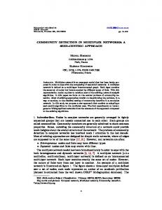
3. Results and discussion 3.1. A synthetic example Consider now a sequence of binary multiplex networks with τ = 30, λ = 5 and ν = 10, generated as follows. Define the perturbation function Π(N, (m, M)) taking as entries a binary simple network N on n nodes, and a couple of real values (m, M) with 0 ≤ m ≤ M ≤ 1, and returning a network N 0 obtained from N by swapping the status (present/not present) of bg n(n−1) 2 c links, where g is a random value in the interval [m, M]. Further, define the default transition as the pair σd = (0.05, 0.2), a small transition as σ s = (0.2, 0.3), a medium transition as σm = (0.25, 0.4) and, finally, a large transition as σl = (0.5, 0.7). Moreover, let R be an Erdós-Rényi G(ν, 0.3) random model and define 4 special timepoints: the initial time step τ0 = 1, the first spike τ1 = 10, the second spike τ2 = 17 and the third spike τ3 = 24. Then, each layer Li at a given time step t is defined through the following rule:    Π(R, σ s ) if t = τ0 and i = 1, 2       Π(R, σm ) if t = τ0 and i = 3, 4       Π(R, σl ) if t = τ0 and i = 5      i  Π(L (t − 1), σ ) if t = τ1 and i = 1, 3, 5  s       or if t = τ2 and i = 3, 5       or if t = τ3 and i = 5  Li (t) =   i  Π(L (t − 1), σm ) if t = τ2 and i = 1, 2        or if t = τ3 and i = 3     i   Π(L (t − 1), σ ) if t = τ1 and i = 2, 4  l      or if t = τ2 and i = 4       or if t = τ3 and i = 1, 2, 4      Π(Li (t − 1), σd ) otherwise . P In Fig. 2 we show the evolution along the 30 timepoints of the 5 curves for D1 (Li ), its average D1 = 15 5i=1 Di (Li ) and D2 , D3 . To assess the information content of each curve we adopt the Increment Entropy (IncEnt) indicator [20], whose value increases with the series’ complexity: the IncEnt values are reported in Tab. 1. Among the evolving layers, L2 and L4 have the largest IncEnt, while the other three layers show a lower level of complexity. As expected, the average D1 and the collapsed network distance D2 has very low IncEnt value, yielding that both averaging the distances and collapsing the layers lose information about the overall dynamics. Finally, distance D3 is the metric which better detects the network evolution along time, conserving most of the information. This is also supported by the changepoints detection indicator mean/variance (meanvar) [19, 25–28], with the CROPS penalty [2 log(τ), 10 log(τ)] [29] in the PELT method [30]. In fact, the meanvar indicator detects correctly in D3 the three points τ1 − 1, τ2 − 1 and τ3 − 1 as changepoints, while in D2 , other than the τ1 − 1, meanvar detects t = 20 and = 28 which are unrelated to the designed dynamics.

Table 1: Increment Entropy values for the distance sequences of the synthetic example, with parameters m = 2, R = 2.

Dist. D1 (L1 ) D1 (L3 ) D1 (L5 ) D2

IncEnt 2.52 2.59 2.44 1.82

Dist. D1 (L2 ) D1 (L4 ) D1 D3 4

IncEnt 2.78 2.83 2.27 3.04

0.4

D1(L1)

0.3

HIM distance

HIM distance

0.4

0.2 0.1

D1(L2)

0.3 0.2 0.1

0

0 2

5

10

15

20

25

30

2

5

10

0.2

25

30

0.1

20

25

30

20

25

30

20

25

30

D1(L4)

0.3 0.2 0.1

0

0 2

5

10

15

20

25

30

2

5

10

Timesteps

0.3

D1(L5)

0.3

15

Timesteps

HIM distance

HIM distance

20

0.4

D1(L3)

0.3

15

Timesteps

HIM distance

HIM distance

Timesteps

0.2 0.1

D1 0.2

0.1

0

0 2

5

10

15

20

25

30

2

5

10

Timesteps

15

Timesteps

0.16

D2

0.12

HIM distance

HIM distance

0.16

0.08 0.04

D3

0.12 0.08 0.04

0

0 2

5

10

15

20

25

30

2

Timesteps

5

10

15

Timesteps

Figure 2: D1 , D2 , D3 for a synthetic example on 5 layers and 30 timepoints; in the right column, third row, we plot D1 =

1 5

P5 i=1

Di (Li ).

3.2. The Gulf Dataset Data description. Part of the Penn State Event Data http://eventdata.psu.edu/ (formerly Kansas Event Data System), available at http://vlado.fmf.uni-lj.si/pub/networks/data/KEDS/, the Gulf Dataset collects, on a monthly bases, political events between pairs of countries focusing on the Gulf region and the Arabian peninsula for the period 15 April 1979 to 31 March 1999, for a total of 240 months. The 304401 political events involve 202 countries and they belong to 66 classes (including for instance ”pessimist comment”, ”meet”, ”formal protest”, ”military engagement”, etc.) as coded by the World Event/Interaction Survey (WEIS) Project [31–33] http://www. icpsr.umich.edu/icpsrweb/ICPSR/studies/5211, whose full list is reported in Tab. 2,3. In the notation of Sec. 2, the Gulf Dataset translates into a time series of τ = 240 multiplex networks with λ = 66 unweighted and undirected layers sharing ν = 202 nodes. The landmark event for the considered zone in the 20 years data range of interest is definitely the First Gulf War (FGW), occurring between August 1990 and March 1999. 5

Table 2: Part 1 of the full table of WEIS codes [31], with the 66 layers considered in the Gulf dataset case study; entries with no layer number were not monitored in the Gulf dataset events collection.

Layer# 1 2 3 4 5 6 7 8 9

10 11 12 13 14 15 16 17 18 19 20 21 22 23 24 25 26 27 28 29 30

31 32 33 34 35

WEIS code 011 012 013 014 015 021 022 023 024 025 026 027 031 032 033 034 041 042 043 051 052 053 054 055 061 062 063 064 065 066 067 070 071 072 073 081 082 083 084 091 092 093 094 095 096 097

WEIS cat Yield Yield Yield Yield Yield Comment Comment Comment Comment Comment Comment Comment Consult Consult Consult Consult Approve Approve Approve Promise Promise Promise Promise Promise Grant Grant Grant Grant Grant Grant Grant Reward Reward Reward Reward Agree Agree Agree Agree Request Request Request Request Request Request Request

Description Surrender, yield or order, submit to arrest, etc. Yield position, retreat; evacuate Admit wrongdoing; retract statement Accommodate, Cease-fire Cede Power Explicit decline to comment Comment on situation – pessimistic Comment on situation – neutral Comment on situation – optimistic Explain policy or future position Appoint or Elect Alter Rules Meet with at neutral site, or send note. Consult & Visit; go to Receive visit; host Vote, Elect Praise, hail, applaud, condole Endorse other’s policy or position; give verbal support Rally Promise own policy support Promise material support Promise other future support action Assure; reassure Promise Rights Express regret; apologize Give state invitation Grant asylum Grant privilege, diplomatic recognition Suspend negative sanctions; truce Release and/or return persons or property Grant Position Reward Extend economic aid (as gift and/or loan) Extend military assistance Give other assistance Make substantive agreement Agree to future action or procedure; agree to meet, to negotiate Ally Merge; Integrate Ask for information Ask for policy assistance Ask for material assistance Request action; call for Entreat; plead; appeal to Request policy change Request rights 6

However, other (smaller) events located in the area had a relevant impact on world politics and diplomatic relations. Among them, the Iraq Disarmament Crisis (IDC) in February 1998 significantly emerges from the data, as shown in what follows. During that month, Iraq President Saddam Hussein negotiated a deal with U.N. Secretary General Kofi Annan, allowing weapons inspectors to return to Baghdad, preventing military action by the United States and Britain.

Table 3: Part 2 of the full table of WEIS codes [31], with the 66 layers considered in the Gulf dataset case study; entries with no layer number were not monitored in the Gulf dataset events collection.

Layer# 36 37 38 39 40 41 42 43 44 45 46

47 48 49 50 51 52 53 54 55 56 57 58 59

60 61 62 63 64 65 66 1

WEIS code 101 102 111 112 113 121 122 123 131 132 133 141 142 150 151 152 160 161 162 171 172 173 174 181 182 191 192 193 194 195 196 197 201 202 203 211 212 213 221 222 223

WEIS cat Propose Propose Reject Reject Reject Accuse Accuse Accuse Protest Protest Protest Deny Deny Demand Demand Demand Warn Warn Warn Threaten Threaten Threaten Threaten Demonstrate Demonstrate Reduce Relations1 Reduce Relations1 Reduce Relations1 Reduce Relations1 Reduce Relations1 Reduce Relations1 Reduce Relations1 Expel Expel Expel Seize Seize Seize Force Force Force

Description Offer proposal Urge or suggest action or policy Turn down proposal; reject protest demand, threat, etc Refuse; oppose; refuse to allow Defy law Charge; criticize; blame; disapprove Denounce; denigrate; abuse Investigate Make complaint (not formal) Make formal complaint or protest Symbolic act Deny an accusation Deny an attributed policy, action role or position Issue order or command; insist; demand compliance; etc Issue Command Claim Rights Give warning Warn of policies Warn of problem Threat without specific negative sanctions Threat with specific non-military negative sanctions Threat with force specified Ultimatum; threat with negative sanctions and time limit specified Non-military demonstration; to walk out on Armed force mobilization Cancel or postpone planned event Reduce routine international activity; recall officials; etc Reduce or halt aid Halt negotiations Break diplomatic relations Strike Censor Order personnel out of country Expel organization or group Ban Organization Seize position or possessions Detain or arrest person(s) Hijack; Kidnap Non-injury obstructive act Non-military injury-destruction Military engagement

as negative sanctions

7

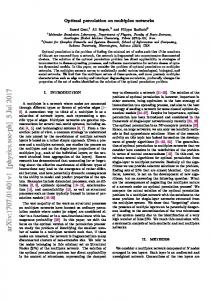
3.3. Network statistics Consider in this section the set of 304401 edges connecting the 202 nodes independently of their class. In Tab. 4 we list the top-10 countries/institutions participating in the largest number of edges across different time spans, together with the absolute number of shared edges and the corresponding percentage over the total number of edges for the period. In general, USA, Iraq and Iran are the major players, with different proportions according to the specific period: in particular, Iraq is the main character in both the major events, FGW and IDC. Other key actors are Israel, the United Nations and the Saudi Arabia, with a relevant presence in each key event in the area. Note that, overall, the top 20 institutions (also including, other than those listed in the table, the Arab world, France, Syria, Egypt, Russia, Turkey, Jordan, Libya, Germany and the Kurd world) are responsible for 82.57% of all edges. = 20301 unique edges, only 4394 are represented in the Gulf Dataset. In Tab. 5 we list Out of all potential 202·201 2 the top-10 links ranked by occurrence, together with the number of occurrences itself and the corresponding percentage over the total number of edges for the period. As it happens for the nodes, there are a few key links throughout the whole timespan which are consistently present in most of the important events, with different proportions. However, in some of the events, there is an interesting wide gap in the number of occurrences between the very top edges and the remaining ones, e.g., Iraq-USA in FGW (and post) and IDC, and Iran-Iraq during the corresponding war and in the pre-FGW, yielding that these are the links mainly driving the whole network evolution. In Fig. 3 we display the dynamics of the occurrence along time of the top edges, showing their different trends during the diverse events. It is interesting to note how two top links, Iran-Iraq and Iran-USA are preponderant from 1979 to 1989, i.e., throughout the whole Iran-Iraq War, while they go decaying quickly afterwards, with a minor spike for FGW. Complementarily, two other major links Iraq-USA and Iraq-United Nations have the opposite trend,

Table 4: Top-10 countries/institutions ranked by number of shared links, absolute and in percentage over (twice) the total number of links in the considered period. The Iran-Iraq War started in September 1980 and ended in August 1988. SA: Saudi Arabia; UN: United Nations.

Apr79-Mar99 Edges 304401 Inst. Degree USA 93900 Iraq 84974 Iran 61782 Israel 32204 UN 30097 SA 20503 Lebanon 19130 Palestine 18607 UK 18415 Kuwait 17405 Apr79-FGW Edges 130990 Inst. Degree Iran 43818 USA 34710 Iraq 25606 Israel 12731 Palestine 10622 Lebanon 10374 SA 10290 Arab world 8237 Syria 8089 UN 6876

% 15.42 13.96 10.15 5.29 4.94 3.37 3.14 3.06 3.02 2.86

% 16.73 13.25 9.77 4.86 4.05 3.96 3.93 3.14 3.09 2.62

FGW Edges 41181 Inst. Degree Iraq 18691 USA 15584 Kuwait 5245 SA 3548 Israel 3420 UN 3363 UK 2997 Iran 2104 France 2076 Arab world 2053 FGW-Mar99 Edges 132230 Inst. Degree USA 43606 Iraq 40677 UN 19858 Israel 16053 Iran 15860 UK 9209 Lebanon 8143 France 6925 Russia 6875 SA 6665

8

% 22.69 18.92 6.37 4.31 4.15 4.08 3.64 2.55 2.52 2.49

% 16.49 15.38 7.51 6.07 6.00 3.48 3.08 2.62 2.60 2.52

IDC Edges 7712 Inst. Degree Iraq 3830 USA 2876 UN 1946 Russia 896 UK 715 France 651 Iran 468 Arab world 321 China 309 Kuwait 306 Iran-Iraq War Edges 95189 Inst. Degree Iran 32812 USA 24111 Iraq 21019 Israel 9189 SA 8089 Palestine 7521 Lebanon 6992 Syria 6072 Arab world 5726 Kuwait 4890

% 24.83 18.65 12.62 5.81 4.64 4.22 3.03 2.08 2.00 1.98

% 17.24 12.66 11.04 4.83 4.25 3.95 3.67 3.19 3.01 2.57

remaining almost uninfluential until FGW and growing later on, with a noticeable spike for IDC; moreover, IraqUnited Nations does not show any trend change for FGW, while Iraq-USA does. The Iraq-Kuwait link has a very limited dynamics, with the unique important spike for FGW. Very similar are also the Saudi Arabia-USA and the Israel-USA links, showing an additional lower spike in correspondence of the raise of the terroristic actions between 1995-1996. This last event is crucial in the Israel-Lebanon relations, where it has the largest effect; FGW, instead, has almost no impact here. D∗ indicators analysis. The two main events FGW and IDC generate sudden changes in the D1 time series for most of the layers: an example is given in Fig. 7 for the layer 37, corresponding to WEIS code 102 (“Urge or suggest action or policy”), where we highlight FGW by a blue background, and IDC by a red dashed line. The complete panel of the D1 curves for all the 66 layers is shown in Fig. 4-6: most of the layers show a decise change in trend in correspondence of the two main events, although some of the layers display a different behaviour (e.g., layer 59, “Break diplomatic relations”), sometimes due to the paucity of data (e.g., “Halt negotiations” or “Reward”). Note that many other spikes exist in many layers, corresponding to different geopolitical events occurring throughout the considered timespan. All the information conveyed by the 66 D1 time series can be summarized by using the D2 and D3 indicators displayed in Fig 8. The two curves show a similar trend, with two major spikes corresponding to the FGW and the IDC, neatly emerging in both time series. Furthermore, both indicators are consistent in showing that the two periods pre- and post-FGW are not part of the FGW spike, implying that in these two periods the structure of the occuring binary geopolitical events is closer to the analogous structure for the “no-war” periods. However, as expected, the indicator D2 includes a lower level of information than D3 : this is particularly evident (also for the smoothed curves, in black in the plots) in the periods 85-89 and 95-97, where the dynamics of D2 is much

Table 5: Top-10 countries/institutions ranked by number of shared links, absolute and in percentage over (twice) the total number of links in the considered period. The Iran-Iraq War started in September 1980 and ended in August 1988. SA: Saudi Arabia; UN: United Nations.

Apr79-Mar99 Edges 304401 Edge Degree Iran-Iraq 19121 Iraq-USA 19002 Iran-USA 14051 Iraq-UN 12775 Israel-Lebanon 6590 Israel-USA 5803 Iraq-Kuwait 5187 SA-USA 4468 Israel-Palestina 4466 UN-USA 4209 Apr79-FGW Edges 130990 Edge Degree Iran-Iraq 16015 Iran-USA 9928 Israel-USA 2714 Iran-UN 2105 Israel-Lebanon 1981 Israel-Palestina 1932 Lebanon-USA 1722 Lebanon-Syria 1591 SA-USA 1554 France-Iran 1418

% 6.28 6.24 4.62 4.20 2.16 1.91 1.70 1.47 1.47 1.38

% 12.23 7.58 2.07 1.61 1.51 1.47 1.31 1.21 1.19 1.08

FGW Edges 41181 Edge Degree Iraq-USA 6061 Iraq-Kuwait 2306 SA-USA 1169 Iraq-UN 1118 Kuwait-USA 1050 Iraq-UK 1012 Iran-Iraq 989 Israel-USA 935 Iraq-Israel 851 Iraq-SA 796 FGW-Mar99 Edges 132230 Edge Degree Iraq-USA 11647 Iraq-UN 10605 Israel-Lebanon 4471 Iran-USA 3797 UN-USA 2575 Iraq-Kuwait 2371 UK-USA 2206 Israel-USA 2154 Israel-Palestina 2144 Iran-Iraq 2117 9

% 14.72 5.60 2.84 2.71 2.55 2.46 2.40 2.27 2.07 1.93

% 8.81 8.02 3.38 2.87 1.95 1.79 1.67 1.63 1.62 1.60

IDC Edges 7712 Edge Degree Iraq-USA 1021 Iraq-UN 927 UN-USA 337 Iraq-Russia 315 Iraq-UK 241 France-Iraq 191 UK-USA 184 France-UN 171 Russia-USA 170 Iraq-Turkey 136 Iran-Iraq War Edges 95189 Edge Degree Iran-Iraq 14470 Iran-USA 6456 Israel-USA 2124 Iran-UN 1402 Israel-Lebanon 1391 Lebanon-USA 1327 SA-USA 1271 Israel-Palestina 1247 France-Iran 1193 Lebanon-Syria 999

% 13.24 12.02 4.37 4.08 3.12 2.48 2.39 2.22 2.20 1.76

% 15.20 6.78 2.23 1.47 1.46 1.39 1.34 1.31 1.25 1.05

Link occurrences

Link occurrences

Iran − Iraq

500 400 300 200 100

1200

Iraq − USA

900 600 300

0

0 04_79

08_82

12_85

04_89

08_92

12_95

03_99

04_79

08_82

12_85

600

Iran − USA

450 300 150

04_79

08_82

12_85

04_89

08_92

12_95

750

08_92

12_95

03_99

08_92

12_95

03_99

08_92

12_95

03_99

Iraq − United Nations

450 300 150

04_79

08_82

12_85

04_89

Date

600

Link occurrences

Link occurrences

03_99

600

03_99

Israel − Lebanon

400 300 200 100 0

Israel − USA

300 200 100 0

04_79

08_82

12_85

04_89

08_92

12_95

03_99

04_79

08_82

12_85

Date

04_89

Date

600

Link occurrences

Link occurrences

12_95

900

Date

500

08_92

0

0

500

04_89

Date

Link occurrences

Link occurrences

Date

Iraq − Kuwait

400 300 200 100 0

300

Saudi Arabia − USA

200 100 0

04_79

08_82

12_85

04_89

08_92

12_95

03_99

04_79

Date

08_82

12_85

04_89

Date

Figure 3: Occurrences along time of the top-8 most frequent links. The blue area marks FGW, while the red dashed line indicates IDC in February 98.

flatter than the dynamics of D3 . Note that a non trivial dynamics in the two periods 85-89 and 95-97 exist in many layers, as shown in Fig. 4-6, triggered by a number of important events impacting the geopolitical relations: the final part of the Iran-Iraq War (1980-1988), the decline and fall of the Soviet Empire (not direclty related to the Middle East area, but reflecting also there), the dramatic change of the situation of the Middle East conflicts induced by the outbreak of the First Intifada in December 1987 [34], and the terrorism excalation (Dhahran, Tel Aviv, and Jerusalem) in Middle East in 95/96 causing a bursting increase in the number of victims just to name the more relevant events. Thus, this case study, too supports the superiority of D3 as a global indicator to summarize the evolution of a series of multiplex networks. 10

n o HIM distances for D (respectively, D ) HIM(CN(t ), CN(t )) We also computed all the 240·239 (resp. 2 3 i j 2 1≤i≤ j≤τ=240 n o HIM(LN(ti ), LN(t j )) ), which are then used to project the 240 networks on a plane through a multidimen1≤i≤ j≤τ=240 sional scaling [36]: the resulting plots are displayed in Fig. 9. Both indicators yield that the months corresponding to FGW (in blue in the plots) are close together and confined in the lower left corner of the plane, showing both a mutual high degree of homogeneity and, at the same time, a relevant difference to the graphs of all other months. Interestingly, this holds also for the months immediately before and after (in green and orange in the figures) the conflict, which are quite distant from the war months’ cloud, as previously observed. This confirms that, only at the onset of the conflict the diplomatic relations worldwide changed consistently and their structure remained very similar throughout the whole event. From both the multidimensional scaling plots in Fig. 9 it is clear that the both the CN and LN networks for the FGW months can be easily discriminated from all other nets. However, from the MDS projections it is not evident whether the months Apr 1979 - Dec 1989 (in grey) could be separated from the Nov 91 - Dec 99 months. By using a Support Vector Machine classifier with the HIM kernel [9, 24] (with γ = 172.9 for LN and γ = 110 for CN), a 5-fold CV classification gives as best result the accuracy 81.2% for LN (C = 103 ) and 73.3% for CN (C = 104 ). Thus, in both cases, machine learning provides a good separation between the networks belonging to the two periods. Community structure of LN. We conclude by analyzing the dynamics of the mesostructure of the layer network LN as extracted by the Louvain community detection algorithm [37–40]. For any temporal step, the Louvain algorithm clusters the 66 nodes (WEIS categories) of LN into two or three communities, whose dimension along time is shown in Fig. 10. In Fig. 11 we show, for each date, which community each category (on the rows) belongs to; WEIS categories are ranked according to their community distribution, i.e., decreasing number of presences in Comm. #1 and increasing for Comm. #2. Thus in top rows we have the categories lying in Comm. #1 during all the 240 months (layers 7,10,11,28,34,40), while bottom rows are reserved to the categories always belonging to Comm. #2 (3,4,19,25,48,52,58): their description in terms of WEIS categories is shown in Tab. 7, while the full community distribution is reported in Tab. 6. Focussing on the categories that are consistently lying in a given community throughout all 240 months, some of them are semantically similar: for instance, consult, assistance, action request in community #1 while two distinct groups emerge in community #2, namely admit wrongdoing, cede power, apologize, reward on one side and warn of policies, sanction threats and halt negotiations characterizing the second group. However, it is interesting the constant presence of the category charge/criticize/blame/disapprove in community #1. Many layers sharing the same (or similar) WEIS second level category (Yield, Comment, Consult, etc.) are quite close in the community distribution ranked list, with a general escalating trend proceedings from help request (or other more neutral actions) to more severe situations growing together with the community distribution rank. 4. Conclusion We introduced here a novel approach for the longitudinal analysis of a time series of multiplex networks, defined by mean of a metric transformation conveying the information carried by all layers into a single network for each timestamp, with the original layers as nodes. The transformation is induced by the Hamming-Ipsen-Mikhailov distance between graph sharing the same nodes, and it preserves the key events encoded into each instance of the multiplex network time series, making it more efficient than the collapsing of all layers into one collecting all edges for detecting inportant fluctuations in the original network’s dynamics. Moreover, a community detection analysis on the obtained network can help shading light on the relations between the original layers throughout the whole time span. References [1] S. Boccaletti, G. Bianconi, R. Criado, C. del Genio, J. Gómez-Gardeñes, M. Romance, I. Sendiña-Nadal, Z. Wang, M. Zanin, The structure and dynamics of multilayer networks, Physics Reports 544 (1) (2014) 1–122. [2] M. De Domenico, A. Solé-Ribalta, E. Cozzo, M. Kivelä, Y. Moreno, M. Porter, S. Gómez, A. Arenas, Mathematical Formulation of Multilayer Networks, Physical Review X 3 (2013) 041022. [3] M. Kivelä, A. Arenas, M. Barthelemy, J. Gleeson, Y. Moreno, M. Porter, Multilayer networks, Journal of Complex Networks 2 (3) (2014) 203–271.

11

Table 6: Community distribution for the 66 WEIS categories: for each layer, we report the number of occurences in the three detected communities.

Rank 1 2 3 4 5 6 7 8 9 10 11 12 13 14 15 16 17 18 19 20 21 22 23 24 25 26 27 28 29 30 31 32 33

[4] [5] [6] [7] [8] [9] [10] [11] [12] [13] [14] [15]

Layer 7 10 11 28 34 40 66 9 37 38 29 30 6 35 41 39 43 14 62 63 2 56 46 36 55 45 64 65 31 22 54 13 49

#1 240 240 240 240 240 240 239 236 234 234 233 232 230 230 222 220 208 196 175 170 164 150 148 146 136 122 121 119 116 110 109 97 97

#2 0 0 0 0 0 0 0 0 2 1 2 2 2 0 3 7 12 18 29 32 28 51 49 48 46 64 71 64 64 79 86 91 80

#3 0 0 0 0 0 0 1 4 4 5 5 6 8 10 15 13 20 26 36 38 48 39 43 46 58 54 48 57 60 51 45 52 63

Rank 34 35 36 37 38 39 40 41 42 43 44 45 46 47 48 49 50 51 52 53 54 55 56 57 58 59 60 61 62 63 64 65 66

Layer 8 17 24 12 47 27 26 18 42 53 61 51 1 60 57 50 59 23 32 15 16 20 33 5 21 44 3 4 19 25 48 52 58

#1 86 86 71 58 56 54 51 45 31 27 26 21 17 15 14 9 7 5 5 4 2 2 2 1 1 1 0 0 0 0 0 0 0

#2 108 106 130 131 130 140 154 153 170 174 179 182 204 204 214 221 225 219 231 232 236 236 237 235 238 231 240 240 240 240 240 240 240

#3 46 48 39 51 54 46 35 42 39 39 35 37 19 21 12 10 8 16 4 4 2 2 1 4 1 8 0 0 0 0 0 0 0

G. Menichetti, D. Remondini, P. Panzarasa, R. Mondragón, G. Bianconi, Weighted Multiplex Networks, PLoS ONE 9 (6) (2014) e97857. L. Weiyi, C. Lingli, H. Guangmin, Mining Essential Relationships under Multiplex Networks, arXiv:1511.09134 (2015). L. Lacasa, V. Nicosia, V. Latora, Network structure of multivariate time series, Nature Scientific Reports 5 (2015) Article number: 15508. K.-M. Lee, B. Min, K.-I. Goh, Towards real-world complexity: an introduction to multiplex networks, The European Physical Journal B 88 (2) (2015) 48. J. Iacovacci, Z. Wu, G. Bianconi, Mesoscopic structures reveal the network between the layers of multiplex data sets, Physics Review E 92 (2015) 042806. G. Jurman, R. Visintainer, M. Filosi, S. Riccadonna, C. Furlanello, The HIM glocal metric and kernel for network comparison and classification, in: Proc. IEEE DSAA’15, Vol. 36678, IEEE, 2015, pp. 1–10. T. Furlanello, M. Cristoforetti, C. Furlanello, G. Jurman, Sparse Predictive Structure of Deconvolved Functional Brain Networks, arXiv:1310.6547 (2013). M. Mina, R. Boldrini, A. Citti, P. Romania, V. D’Alicandro, M. De Ioris, A. Castellano, C. Furlanello, F. Locatelli, D. Fruci, Tumor-infiltrating T lymphocytes improve clinical outcome of therapy-resistant neuroblastoma, OncoImmunology 4 (9) (2015) e1019981. D. Fay, A. Moore, K. Brown, M. Filosi, G. Jurman, Graph metrics as summary statistics for Approximate Bayesian Computation with application to network model parameter estimation, Journal of Complex Networks 3 (2015) 52–83. A. Gobbi, G. Jurman, A null model for Pearson correlation networks, PLoS ONE 10 (6) (2015) e0128115. S. Masecchia, Statistical learning methods for high dimensional genomic data, Ph.D. thesis, DIBRIS, University of Genua (2013). P. Csermely, T. Korcsmáros, H. Kiss, G. London, R. Nussinov, Structure and dynamics of biological networks: a novel paradigm of drug

12

Table 7: The 13 layers not swapping community across all 240 timepoints.

Layer 7 10 11 28 34 40

WEIS code 023 031 032 073 094 121

Layer 3 4 19 25 48 52 58

WEIS code 013 015 061 070 161 174 194

Community #1 WEIS category [Comment] Comment on situation neutral [Consult] Meet with at neutral site, or send note [Consult] Consult & Visit; go to [Reward] Give other assistance [Request] Request action; call for [Accuse] Charge; criticize; blame; disapprove Community #2 WEIS category [Yield] Admit wrongdoing; retract statement [Yield] Cede power [Grant] Express regret; apologize [Reward] Reward [Warn] Warn of policies [Threaten] Ultimatum; threat with negative sanctions and time limit specified [Reduce Relations] Halt negotiations

discovery. A comprehensive review, Pharmacology and Therapeutics 138 (2013) 333–408. [16] M. De Domenico, V. Nicosia, A. Arenas, V. Latora, Structural reducibility of multilayer networks, Nature Communications 6 (2015) 6864. [17] A. Cardillo, J. Gómez-Gardeñes, M. Zanin, M. Romance, D. Papo, F. del Pozo, S. Boccaletti, Emergence of network features from multiplexity, Nature Scientific Reports 3 (2013) Article number: 1344. [18] Y. Takenaka, S. Seno, H. Matsuda, Detecting shifts in gene regulatory networks during time-course experiments at single-time-point temporal resolution, Journal of Bioinformatics and Computational Biology 13 (5) (2015) 1543002–1:18. [19] R. Killick, I. Eckley, changepoint: An R Package for Changepoint Analysis, Journal of Statistical Software 58 (1) (2014) 1–19. [20] X. Liu, A. Jiang, N. Xu, J. Xue, Increment entropy as a measure of complexity for time series, arXiv:1503.01053 (2015). [21] A. Schein, J. Moore, H. Wallach, Inferring Multilateral Relations from Dynamic Pairwise Interactions, arXiv:1311.3982 (2013). [22] A. Schein, J. Paisley, D. Blei, H. Wallach, Bayesian Poisson Tensor Factorization for Inferring Multilateral Relations from Sparse Dyadic Event Counts, in: Proc. KDD 2015, ACM, 2015, pp. 1045–1054. [23] M. Jackson, S. Nei, Networks of military alliances, wars, and international trade, Proceedings of the National Academy of Sciences 112 (50) (2015) 15277–15284. [24] G. Jurman, R. Visintainer, S. Riccadonna, M. Filosi, C. Furlanello, The HIM glocal metric and kernel for network comparison and classification, arXiv:1201.2931v3 (2014). [25] J. Chen, A. Gupta, Parametric Statistical Change Point Analysis, Springer, 2012. [26] A. Scott, M. Knott, A Cluster Analysis Method for Grouping Means in the Analysis of Variance, Biometrics 30 (3) (1974) 507–512. [27] I. Auger, C. Lawrence, Algorithms for the Optimal Identification of Segment Neighborhoods, Bulletin of Mathematical Biology 51 (1) (1989) 39–54. [28] N. Zhang, D. Siegmund, A Modified Bayes Information Criterion with Applications to the Analysis of Comparative Genomic Hybridization Data, Biometrics 63 (2007) 22–32. [29] K. Haynes, I. Eckley, P. Fearnhead, Efficient penalty search for multiple changepoint problems, arXiv:1412.3617 (2014). [30] R. Killick, P. Fearnhead, I. Eckley, Optimal detection of changepoints with a linear computational cost, Journal of the American Statistical Association 107 (500) (2012) 1590–1598. [31] C. McClelland, World Event/Interaction Survey Codebook, Vol. 5211 of ICPSR, Inter-University Consortium for Political and Social Research, Ann Arbor, 1976. [32] J. Goldstein, J. Pevehouse, International Cooperation and Regional Conflicts in the Post-Cold War World, 1987-1999, Tech. Rep. ICPSR02761-v1, Inter-university Consortium for Political and Social Research [distributor], Ann Arbor, MI (2004). [33] J. Goldstein, A Conflict-Cooperation Scale for WEIS Events Data, The Journal of Conflict Resolution 36 (2) (1992) 369–385. [34] R. Ragionieri, The Peace Process in the Middle East: Israelis and Palestinians, The International Journal of Peace Studies 2 (2). [35] J. Durbin, S. Koopman, Time Series Analysis by State Space Methods, Oxford University Press, 2001. [36] T. Cox, M. Cox, Multidimensional Scaling, Chapman and Hall, 2001. [37] V. Blondel, J.-L. Guillaume, R. Lambiotte, E. Lefebvre, Fast unfolding of communities in large networks, Journal of Statistical Mechanics: Theory and Experiment 10 (2008) P10008. [38] A. Lancichinetti, S. Fortunato, Community detection algorithms: a comparative analysis, Phys. Rev. E 80 (2009) 056117. [39] T. Aynaud, V. Blondel, J.-L. Guillaume, R. Lambiotte, Optimisation locale multi-niveaux de la modularité, in: C.-E. Bichot, P. Siarry (Eds.), Partitionnement de graphe Optimisation et applications, Hermes Paris, 2010, p. 14. [40] A. Lancichinetti, S. Fortunato, Consensus clustering in complex networks, Nature Scientific Reports 2 (2012) Article number: 336.

13

SURRENDER

RETREAT

RETRACT

CEDE POWER

DECLINE COMMENT

PESSIMIST COMMENT

NEUTRAL COMMENT

OPTIMIST COMMENT

EXPLAIN POSITION

MEET

VISIT

RECEIVE

PRAISE

ENDORSE

PROMISE POLICY SUPPORT

PROMISE MATL SUPPORT

PROMISE OTHER SUPPORT

ASSURE

APOLOGIZE

STATE INVITATION

GRANT ASYLUM

GRANT PRIVILEGE

TRUCE

RELEASE

Figure 4: Curves of indicator D1 for the 24 layers Li (t), for i = 1, . . . , 24: the blue area marks FGW, while the red dashed line indicates IDC in February 98. For each curve, the corresponding World Event/Interaction Survey category is indicated in the top left corner.

14

REWARD

EXTEND ECON AID

EXTEND MIL AID

GIVE OTHER ASSIST

MAKE AGREEMENT

AGREE FUTURE ACT

ASK INFORMATION

ASK POLICY AID

ASK MATERIAL AID

CALL FOR

PLEAD

OFFER PROPOSAL

URGE

TURN DOWN

REFUSE

CRITICIZE

DENIGRATE, DENOUNCE

MAKE COMPLAINT

FORMAL PROTEST

DENY ACCUSATION

DENY ACTION


15

DEMAND

WARN

WARN POLICIES

UNSPECIFIED THREAT

NONMIL THREAT

SPECIF THREAT

ULTIMATUM

NONMIL DEMO

MILITARY DEMO

CANCEL EVENT

CUT ROUTINE ACT

CUT AID

HALT NEGOTIATION

BREAK DIPL RELAT

EXPEL PERSONNEL

EXPEL GROUP

SEIZE POSSESSION

ARREST PERSON

NONINJURY DESTR

NONMILITARY DESTR

MILITARY ENGAGEMENT


16

HIM distance

0.12

102 Urge or suggest action or policy

0.08

0.04

0 04_79

04_81

04_83

04_85

04_87

04_89

04_91

04_93

04_95

04_97 03_99

Date Figure 7: D1 time series for the layer 37, corresponding to WEIS code 102 (“Urge or suggest action or policy”). The period corresponding to FGW is marked by the blue background, while the red dashed line indicates IDC in February 1998.

17

0.16

HIM distance

0.12

Apr79 − Dec89 Jan90 − Jul90 Gulf War Apr91 − Oct91 Nov91 − Dec99 Smoothed

Feb 98 ●

0.08

0.04

0 04_79

04_81

04_83

04_85

04_87

04_89

04_91

04_93

04_95

04_97

03_99

Date

HIM distance

0.12

0.08

Apr79 − Dec89 Jan90 − Jul90 Gulf War Apr91 − Oct91 Nov91 − Dec99 Smoothed

Feb 98 ●

0.04

0 04_79

04_81

04_83

04_85

04_87

04_89

04_91

04_93

04_95

04_97

03_99

Date

Figure 8: Time evolution of a global view of the (monthly) Gulf Dataset. (top) D2 dynamics of the collapsed projections {CN(t)}240 t=1 and (bottom) D3 dynamics of the metric projections {LN(t)}240 t=1 . For each date, the value on y-axis the is the HIM distance from the first element of the time series. Different colors mark different time periods. The black line represents the fixed-interval smoothing via a state-space model [35].

18

● ● ● ● ●

●

● ● ● ● ● ● ● ● ● ● ● ● ● ● ● ●● ● ●● ● ● ● ● ● ● ●● ● ●●● ● ● ● ●● ● ●● ● ● ●● ● ● ● ● ● ● ● ● ● ● ● ●●● ● ● ● ●● ● ●● ●● ● ● ●●● ● ● ●● ● ●● ● ● ● ● ● ●● ●● ●● ● ● ● ● ● ● ● ● ●● ●● ● ●●● ● ●● ● ● ● ● ●● ● ● ● ● ● ● ● ● ● ● ●● ● ● ● ● ● ● ● ● ● ● ● ● ● ● ● ● ● ● ● ● ● ● ● ● ● ● ● ● ● ● ● ● ● ● ● ● ●●●● ●● ● ● ● ●●● ● ● ●● ● ● ●● ●●● ● ● ● ●● ●● ● ● ● ● ● ● ● ● ● ● ●● ● ● ● ●● ● ● ● ● ● ●● ● ● ●● ● ●

0.02

●

0.00

−0.02

● ●

−0.04

● ●

Apr79 − Dec89 Jan90 − Jul90

● ●

Gulf War Apr91 − Oct91

−0.05

0.005

0.000

−0.005

−0.010

−0.015

● ●

Feb98 Nov91 − Dec99

0.00

●

0.05

0.10

● ●● ● ● ● ● ● ● ●● ● ● ● ●● ● ● ●● ● ● ● ●● ●● ● ●●●●●● ●● ● ● ● ● ● ● ● ● ● ● ● ● ● ● ● ● ● ● ● ● ● ● ● ● ● ● ● ● ● ● ● ● ● ● ●● ● ● ●●● ● ● ●●● ●● ●●● ● ● ● ● ● ●● ● ● ●● ● ● ● ● ● ● ● ●● ●● ● ● ● ●●●● ● ●●● ● ● ● ● ● ● ● ● ● ● ● ●● ●● ● ● ● ● ● ● ● ● ● ● ● ● ● ● ● ● ● ● ● ● ● ● ● ● ●● ● ●● ●● ●● ● ● ●●● ●● ●●● ●●● ●●● ● ●● ● ● ● ● ● ● ● ●●● ●● ●● ● ● ●●● ●● ●● ● ● ● Apr79 − Dec89 ● Jan90 − Jul90 ● Gulf War ● Apr91 − Oct91 ● Feb98 ● Nov91 − Dec99

●●

●

● ● ●

● ●

0.00

0.05

0.10

Figure 9: Planar multidimensional scaling plot with HIM distance of the collapsed (top) and metric (bottom) projection for the monthly Gulf Dataset. Colors are consistent with those in Fig. 8.

19

Comm. #1

Comm. #2

Comm. #3

66

Community size

60 50 40 30 20 10 0 04_79

08_82

12_85

04_89

08_92

12_95

03_99

Date Figure 10: Dimension of the three communities indentified by the Louvain algorithm in LN along the 240 months.

20

Comm. #2

Comm. #3

12_85

04_89

08_92

WEIS category

Comm. #1

04_79

08_82

12_95

Date

Figure 11: Community evolution along time for each of the 66 WEIS categories, ranked by community distribution.

21

03_99

14

a

60 1

b

43

23 41 39

57 50 44

= 3,4,19,25,48,52,58

5 15 32 1620 2133

= 7,10,11,28,34,40

66

49

c 47 12 51 6153 42

35 6 30 29 38 37 9

59

18 26

13

17 8

27

22 54

24

31 65 45 64

55 36 46 56

Figure 12: Triangleplot projection of the 66 WEIS categories defined by their community distribution.

22

2 63 62