Miche: Modular Shape Formation by Self-Disassembly - CiteSeerX

Miche: Modular Shape Formation by Self-Disassembly Kyle Gilpin, Keith Kotay, Daniela Rus, and Iuliu Vasilescu

Abstract— We describe the design, implementation, and programming of a set of robots that, starting from an amorphous arrangement, can be assembled into arbitrary shapes and then commanded to self-disassemble in an organized manner, to obtain a goal shape. We present custom hardware, distributed algorithms, and experimental results from hundreds of trails which show the system successfully forming complex threedimensional shapes. Each of the 28 modules in the system is implemented as a 1.8-inch autonomous cube-shaped robot able to connect to and communicate with its immediate neighbors. Embedded microprocessors control each module’s magnetic connection mechanisms and infrared communication interfaces. When assembled into a structure, the modules form a system that can be virtually sculpted using a computer interface and a distributed process. The group of modules collectively decide who is on the final shape and who is not using algorithms that minimize information transmission and storage. Finally, the modules not in the structure disengage their magnetic couplings and fall away under the influence of an external force, in this case, gravity.

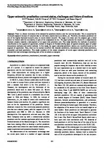
I. I NTRODUCTION We present a modular robotic system named Miche that behaves as programmable matter (see Figure 1). The approach to realizing programmable matter uses selfdisassembly as the fundamental operation to achieve shape formation. The function of self-disassembling modular robots can be thought of as analogous to sculpting. We start with a large block made of individual modules. The initial structure is transformed into the desired shape by eliminating the unnecessary modules from the structure in a controlled fashion. Much like a sculptor would remove the extra stone from a block of marble to reveal a statue, our self-disassembling system eliminates modules to form the goal structure.

Fig. 1. A self-disassembling system can transform from an initial uniform assembly of identical modules, (a), into a more interesting and functional assembly in (b). This work was supported by Intel and Magswitch. K. Gilpin, K. Kotay, D. Rus, and I. Vasilescu are with the Computer Science and Artificial Intelligence Lab, MIT, Cambridge, MA, 02139, [email protected], [email protected], [email protected], [email protected].

The key innovations of our work are (1) the concept of achieving shape formation by self-disassembly; (2) a first hardware prototype capable of self-disassembly; and (3) a suite of provably correct distributed algorithms capable of planning and controlling self-disassembly in an optimal manner that minimizes information flow. The Miche system serves as a hardware proof of concept and a testbed for distributed algorithm development. The algorithms were developed with the expectation that the physical size of individual modular robots will shrink and the number of robots in modular systems will grow. Efficient algorithms that pass a minimal number of messages will become a necessity as modular systems become increasingly dense. Creating robotic systems and smart objects by selfdisassembly has one main advantage over existing approaches by self-assembly. Self-disassembling systems entail a simple actuation mechanism (disconnection) which is generally easier, faster, and more robust than actively seeking and making connections. The trade-off is three-fold. First, self-disassembling systems must start from a pre-assembled structure of modules. In our work, this block is assembled manually, but this process can be automated using mechanical fixtures. Although this process requires some additional effort, assembling the initial block, (due to its regularity), is easier than immediately forming the more complex goal structure. As additional modules are brought into contact with the initial block, the modules already present provide a rapid and reliable means of alignment. Furthermore, until a module is aligned with its neighbors, it remains unbound and free to continue moving. With the help of external environmental forces, it may even be possible for unbound modules to self-assemble an initial block of material. The second trade-off associated with actuation by disconnection is that external forces must be employed to remove unwanted material from the system. Often, these forces can be found in the surrounding environment. For our experiments, we used gravity to pull unnecessary modules away from the final structure. Third, unlike most self-assembling system, self-disassembling systems, because their only method of actuation is disconnection, cannot reconfigure themselves without jettisoning some number of modules. Modular robots that can self-disassemble provide a simple and robust approach toward the goal of smart structures and digital clay. A collection of millions of modules, if each were small enough, could form a completely malleable building material that could solidify and then disassemble on command. As in existing selective laser sintering systems, (which fuse particulate matter to create rapid prototypes), a selfdisassembling robotic system would only require the user to

shake off the unused modules. A plethora of intelligent and interactive objects could be created through this process of organized disassembly and removal of extra material. The applications of self-disassembling systems include entertainment, object creation by programmable matter, 3d printing and rapid prototyping, and all the other applications of self-assembling systems. Specific modules could be equipped with specialized actuators or sensors. After the self-disassembly process completes, the these actuators could be employed for additional locomotion or manipulation. The added flexibility of removing specific components from the assembly ensures that our approach is especially well suited to tasks requiring temporary supporting structures. For example, self-disassembling material could be applied as an active scaffolding to help heal severely broken bones that would otherwise require the use of permanent steel plates or pins. In addition to disassembling as the bone regrows, the scaffolding could provide valuable medical status information to doctors. In such a scenario, the bloodstream could carry away extra modules. The first part of this paper is devoted to describing the Miche hardware that we designed and built. Each module is a cube whose faces are the PCBs used for the electronics and control of the system. (Although we chose identically sized modules, the system could be adapted to employ completely passive modules as well as modules that were integer multiples of the fundamental unit size.) Each module has on-board computation and power, point-to-point IR communication with its immediate neighbors, and three switchable permanent magnets. These magnets provide the connection between adjacent units and have the feature of activating or deactivating depending on their orientation. Three small motors capable of rotating the magnets provide the disconnection actuation in the system. We have built a system consisting of 28 Miche modules. The second part of this paper describes the algorithms employed to achieve shape formation by self-disassembly. Shape formation with Miche modules proceeds as follows. First, an initial amorphous shape is assembled by hand (e.g. see Figure 1(a)). The modules in this initial structure use local communication to establish their location within a system of coordinates. After the initial configuration has been assembled, the user provides a goal shape for the system. Using local communication, the group cooperates to distribute this information so that all modules know whether to remain as a part of the system or to extricate themselves. Finally, the unnecessary modules disconnect from the system and drop off to create the desired shape (e.g. see Figure 1(b).) After describing the the hardware, algorithms, and systems issues associated with achieving such a distributed system, this paper presents our initial experimental results. The system exhibits very reliable behavior. We believe this is due to the actuation method employed for shape formation because it does not have to solve the challenging task of forming precise inter-module connections.

A. Related Work Our work draws on prior and ongoing research in modular and distributed robotics [YZR+ 03], [CBW02], [KKY+ 05], [RV03], [CW00], [PEUC97], [UK00], [Yim], [WZBL05], [BKGS06], [PCK+ 06] and self-assembling systems [Nag02], [WG02]. Most these systems are composed of identical modules that can connect to each other, communicate, have some actuation capabilities, and in general are able to cooperate to perform a task as a group. Like in these prior systems, our modules can connect and communicate with each other in order to perform a global task. Our connection mechanism is novel however and has some advantages. Previous systems use mechanical connections actuated by shape-memory alloys (SMA) [YZR+ 03], [CBW02], [UK00], or by electric motors [RV03], electromagnetic connections [WZBL05], static permanent magnet connections [Yim] or SMA actuated [KKY+ 05] or SMA springs [YMK+ 02], [YKM+ 01]. A novel system for self-assembly and reconfiguration is presented by White [WZBL05] which uses fluid flow to bind individual modules together. In [PCK+ 06], Pillai et. al. simulate using thousands of mechanically passive modules to construct digital representations of three-dimensional objects. The CHOBIE robot developed by Koseki [KMI04] is unique in its mechanical design. The modules in the CHOBIE system, which are also rectangular, are able to locomote by sliding in two planes relative to one another. Unlike the previous mechanical systems, our modules have no protrusions (they are flat faced cubes) and therefore they have less parts to break and are easier to assemble. Compared to SMA and electromagnetic systems, our modules do not use power in any of the states (they only use power for transitions). One key advantage of a switchable magnet connector is that the power used for actuation is almost independent of the final connection force. The previous systems capable of programmable matter are focused on using actuations to change the relative position of the modules in order to achieve their goals. In contrast, the system discussed in this paper creates desired shapes solely by self-disassembly. This requires a suite of novel support algorithms for shape formation, specifically efficient and scalable distribution of shape information across the modules, without, for example, the need of reprogramming the modules as in [Nag02]. The algorithms in this paper have provable time and space complexity limits to ensure they will gracefully scale with the miniaturization of the basic module and increase in the number of modules in the system. II. M ICHE H ARDWARE Figure 2 shows a Miche module prototype. Each module contains the resources necessary for autonomous operation: processing capabilities, actuation mechanisms, communication interfaces, and power supplies. The modules are built from six distinct printed circuit boards that interlock to form a rigid structure. Two groups of three circuit boards each are soldered together to form the two halves of a cube. These two halves then mate using two friction-based electrical connectors so that the cubes can be easily disassembled for

Fig. 4. Each Magswitch consists of two permanent magnets stacked on top of each other inside of a metal housing. The bottom magnet is fixed while the top one contains a keyway and is free to rotate. As the top magnet is rotated through 180o , the entire device switches from on to off or vice versa.

Fig. 2. Each module in the system is a cube which measures 1.77 inches on each side and weighs 4.5oz. Each module is completely autonomous and can operate for several hours under its own power.

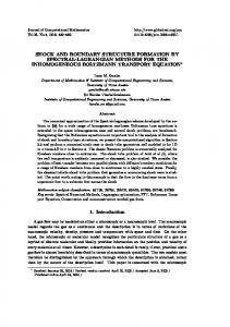
testing and maintenance. When completely assembled, each cubic module is 1.8 inches on a side and weighs 4.5 oz. As shown by an open module in Figure 3, all electronic components are surface mounted on the top side of the boards so that when assembled into cubes, all components reside on the inside. The only pieces of the system mounted externally are three steel plates that form half of the magnetic connection mechanism, presented in detail below. A. Connection Mechanism Individual modules bind to each other using switchable permanent magnet assemblies, hereafter referred to as Magswitches. These assemblies are produced by Magswitch Technology, Inc. [Mag]. Figure 4 shows an example Magswitch. Three of the faces of each cubic module contain Magswitches. Like all other components, they are mounted on the inside of the cubes and pass through similarly sized holes in the printed circuit boards. The other three cube faces of each cube are covered by steel plates. The steel is cold rolled A336/1008 that is 0.033 inches thick. When multiple cubes are assembled into a structure, the Magswitches always attach to the steel plates of a neighboring cube, not one of the other cube’s Magswitches. As a result, the modules can only attract one another. They do not repel but, instead, depend upon gravity or user intervention to clear unused modules from any final structure. A single Magswitch connected to a neighbor’s steel plate can support over 4.5 lbs.—the combined weight of 17 other modules hanging vertically. The Magswitch assemblies control a magnetic field by changing the relative orientation of two permanent disc magnets. The magnet with the keyway shown in the assembly in Figure 4 can rotate freely with respect to the fixed magnet that sits below it in the structure. Depending on the two magnets’ relative orientations, the Magswitch is either

activated and attracts other ferromagnetic materials, or it is deactivated and releases it hold. The Magswitches do not weaken with time because the south poles, (and north poles), of the magnets in each Magswitch are only brought into close proximity when the Magswitch is on and attached to the steel face of a neighboring cube. As a result, the combined magnetic flux has a “low resistance” path from north pole to south. The advantage of using Magswitches for activation is that power is only consumed while changing the state of the Magswitch. Once a Magswitch is on or off, it remains in that state indefinitely. This is invaluable for the battery life of the modules. A miniature pager-sized motor with an integrated planetary gear box drives each Magswitch. These motors have a stall torque of 0.28oz-in [Sol06]. A 17-thread-per-inch worm gear is glued to the motor’s output shaft. This worm gear turns a 30-tooth spur gear which has a key that matches the keyway of the Magswitch shown in Figure 4. The entire motor, worm gear, spur gear, and Magswitch assembly is illustrated in Figure 5. When driven with 4.1V , the voltage of a freshly charged lithium-polymer battery, the motor requires approximately 1.3 seconds to switch a deactivated Magswitch on and back off again.

Fig. 5. A worm gear attached to the output shaft of a miniature DC motor turns a spur gear that mates with the keyway in the Magswitch. In the figure, the Magswitch is obscured by the spur gear, and the removed top cover of the entire assembly is shown on the left.

The motor driver circuit consists of a single MOSFET. As a result, the motor can only turn in one direction, but three additional MOSFETs, which would be needed to run the motor in both directions, are eliminated. The disadvantage to only being able to rotate the Magswitches in one direction is that a motor may stall while activating its Magswitch leaving the Magswitch stranded in a partially activated configuration. (It is not uncommon for a motor to stall if its Magswitch is not in direct contact with a neighboring module’s steel place or some other ferromagnetic material.) If the motor could reverse directions, it would at least be able to return

Fig. 3. An open module shows all of its major components. Each contains two microprocessors, connection mechanisms, infrared emitters and detectors, an accelerometer, a tilt switch, and batteries. Each cube is totally self-sufficient.

its Magswitch to the deactivated state. An analog Hall Effect sensor is used to detect the state of each Magswitch. The Hall Effect sensor is placed such that its axis of sensitivity is aligned with the magnetic field produced by the Magswitch. As the Magswitch rotates, the Hall Effect sensor produces a voltage that approximates a sine wave. B. Processors Each module contains two microprocessors that perform different tasks. The primary microprocessor is a 32-bit ARM processor produced by Philips. It is responsible for all of the high-level disassembly algorithms. The second processor is an 8-bit programmable system on a chip (PSoC) that is manufactured by Cypress Microsystems. The PSoC handles the low-level functions that would otherwise occupy the ARM. In particular, it implements six serial receive ports, one for each face of the module. This allows a single module to receive messages from all its neighbors simultaneously. The ARM and PSoC communicate using the I2 C protocol [Sem00]. C. Communication Interface Communication between modules is performed using infrared light. Each of the six cube faces contains an infrared LED and an infrared sensitive photodiode. Together, these allow bidirectional communication between neighboring cubes at 9600 bits per second (bps). While higher bit rates were achievable, 9600bps proved adequate. Infrared communication has several advantages over other alternatives such as direct electrical contacts. First, an in-

frared based system does not require that the faces of neighboring cubes be completely flush. In an assembly of many modules, this is a legitimate concern because imperfections in the manufacturing process produce cubes that are not perfectly square nor exactly the same size. Electrical contacts would also be disadvantageous because they may short out on the steel plates that cover three of the six cube faces. In order to simplify the design of the circuit boards which compose the faces of the modules, the infrared LED and photodiode were not always placed in the center of each face. This, and the fact that Magswitches must always contact steel plates, dictates that every module has only one valid orientation in a composite structure. Otherwise, the LEDs and photodiodes of neighboring cubes would not align. However, because any self-disassembling structure must be assembled by manually, this restriction does not affect the functionality of the system. The infrared LED and photodiode have both a limited range and a limited field of view. Like all of the electrical components, the LED and photodiode are mounted on the inside faces of the modules, and they point outward through holes in the circuit boards. In order to prevent these holes from further restricting the field of view of the emitters or receivers, they are countersunk from the back (bottom) side of the boards. D. Sensing Each module is able to detect its absolute threedimensional orientation by using a two-axis accelerometer

and a binary tilt switch that are connected to the ARM microprocessor. The accelerometer returns two PWM signals that correspond to the acceleration that each axis is experiencing. The period of these signals is fixed, but the percentage of one period that the signal is on is proportional to acceleration. The ARM microprocessor measures the pulse width of the two signals to obtain an estimate of the cube’s orientation. A tilt switch is needed to disambiguate the data produced by the two-axis accelerometer because the cubes exist and operate in a three-dimensional environment. (The specific two-axis accelerometer used in Miche was chosen for its increased durability in comparison to most three-axis accelerometers.) Like the accelerometer, the tilt switch was also chosen for its durability. Instead of a typical mercury-filled glass cylinder, each tilt switch uses a small metal ball bearing encased in a metal cylinder. While the tilt switch only tells the microprocessor whether the module is oriented roughly up or down, this information, combined with the more precise data from the accelerometer, is enough to determine which side of a module is facing down.

III. L OW-L EVEL C OMMUNICATION

AND

C ONTROL

To support the algorithms that allow our system of modules to disassemble, we have implemented a series of lowlevel functions that control the hardware in each module. These routines place an abstraction barrier between the localization, shape distribution, and disassembly algorithms and the complex hardware contained in each module. This separation facilitates the rapid implementation and modification of the high-level concepts which are responsible for the system’s visible behavior. The high-level algorithms do not have to contend with the specifics of basic tasks such as exchanging messages or activating a Magswitch. Once a module has the ability to transmit and receive messages, the low-level operation reduces to the simple process illustrated in Figure 6. After initializing, a module loops forever, simply receiving and transmitting messages to its neighbors. The interesting behavior responsible for the system’s self-disassembly is governed by how the highlevel algorithms for shape aggregation respond to received messages.

E. Power Each module is equipped with two rechargeable lithiumpolymer batteries connected in parallel. These batteries supply power to the module’s electronics and motors. They provide 3.7V nominally and have a combined capacity of 340mAh. If the batteries are fully charged and the module is continuously transmitting messages on each face but not running its motors, the usable battery life is over six hours. The batteries drive the motors directly, but two voltage regulators provide power for the electronics. One produces 3.3V which is used by all of the components. The other regulator produces 1.8V which is only used by the core of the ARM microprocessor. The modules can be recharged without removing the batteries. Each module contains an integrated circuit that manages the process. The electrical connection to recharge the batteries is provided through two of the metal faces that adorn the outside of the cubes. Large areas of solder mask are missing on the bottom (outside) of two of the printed circuit boards that form the faces of the cubes in order to electrically connect the steel plates to the circuit. To achieve a reliable connection, the plates are affixed with conductive epoxy. To recharge the batteries, the modules are set in a 28 inch long trough whose metal sides supply a potential difference of 5V. The trough can recharge 15 modules simultaneously. Current to recharge each module’s batteries flows from the sides of the trough, through the metal faces and conductive epoxy to the solder mask-free contacts on the back of the printed circuit boards. The integrated circuit responsible for managing the charging process automatically detects when a charging voltage is present. Therefore, starting or stopping the charging process is achieved by simply placing the modules in, or removing the modules from, the charging trough.

Fig. 6. The message processing loop executing on each module is simple. First, modules initialize all their peripherals. Then, they loop infinitely, receiving and sending inter-module messages. How a module changes its internal state in response to received messages and what messages it transmits in return, dictate the system’s high-level abilities.

All inter-module communications utilize the IR LED and photodiode pairs that exist on each of the module’s six faces. The process of transmitting a message involves several steps. First, the message body is constructed. Then, a checksum produced by a cyclic redundancy check (CRC) is appended to the message. Next, the ARM processor sends a SET TX CHANNEL command over the I2 C interface directing the PSoC to activate the RS-232 transmission multiplexer so that the message is directed to the correct face. After the PSoC acknowledges that it received this command, the ARM sends the message over the RS-232 interface, through the

PSoC, and to the correct IR LED. Finally, once all bits have been transmitted, the ARM once again uses an I2 C bus to deactivate the transmission multiplexer. Messages consist of ASCII characters. They start and end with a special character and have the format shown in Figure 7. msg. type

transmit face #

&

sequence number

start character

&

XXX

one byte

optional type-specific fields CRC & check sum \r

&

cmd. terminator

field delimiter

Fig. 7. Messages are composed of a start character, some number of alphanumeric data fields separated by ampersands, a hexadecimal checksum, and a message terminator.

Receiving messages from neighboring cubes also requires several steps. First, the ARM must use the I2 C bus to configure the digital-to-analog converter that drives the noninverting inputs of a set of comparators attached to the IR photodiodes. (The comparators use this threshold value to convert the analog output of each photodiode to a digital signal.) Once the DAC is configured, it will continue to supply a constant voltage. As a result, this step is only necessary when a module turns on. Assuming that the threshold voltage is reasonable, the ARM proceeds to query the PSoC receive buffers for the presence of any messages using the GET RX STATUS I2 C command. If some buffer contains a valid message, the ARM issues a READ RX BUFFER command to retrieve the message. After the PSoC transfers a message to the ARM, it automatically empties the buffer that had been holding the message. Doing so allows the buffer to once again begin filling with the next message that is received on the specified face. The most important inter-module message types and abbreviations are • acknowledge (ACK) • ping (detect neighbors) (PNG) • localize (LOC) • reflection (inform system of module’s existence) (REF) • include in final structure (INC) • disassemble (DAS) • disconnect request for a specific Magswitch (DRQ) • disconnect all Magswitches (DCA) IV. D ISTRIBUTED C ONTROL

AND

P LANNING

These basic inter-module messages are used to drive the high-level control algorithm for self-disassembly which is divided in four phases and shown in Figure 8. Each of the four phases of self-disassembly is dependent on a distributed, localized message passing algorithm executing on each module. The first phase, neighbor discovery, commences after the modules are reset. Modules are added manually to the initial assembly one at a time. During this phase, modules use lowlevel messages to detect any neighbors in close proximity and attempt to establish mechanical and communication links. When a neighbor module is detected on a face, the Magswitch on that face is commanded to rotate to the on

Fig. 8. The entire self-disassembly process consists of four phases: neighbor discovery, localization, shape distribution, and disassembly.

position. At the end of the phase all the modules in the structure are connected as solid block. During the localization phase, which follows neighbor discovery, modules discover their positions within the structure and transmit their positions back to a MATLAB program (see Figure 9) running on the user’s desktop computer. Localization messages are used to efficiently compute relative coordinates for each module in the physical assembly. Once each module has transmitted its position to the user’s computer, the MATLAB program can form and display a model of the system using a GUI. Using this model, the desired final configuration of modules can be virtually sculpted. Using the GUI, the user selects whether each module is included or excluded from the final shape. After this sculpting process is complete, the program generates a sequence of shape distribution messages that is sent to the modules during phase three. During this next shape distribution phase, the modules propagate the inclusion messages generated by the GUI. The fourth, and final, phase is disassembly. During the disassembly phase the modules not in the final shape disconnect from the system to reveal the shape the user sculpted using the GUI. The entire self-disassembly process showing the GUI and the modular structure side-by-side can be seen in Extension 1. One important goal for the self-disassembly algorithms was to compress required shape description information per module and to minimize the required number of point-topoint messages. Our decentralized approach is in contrast to the centralized approach where the entire shape description is given to each module using global messages that can flood the entire structure. The centralized approach does not scale with respect to the number of modules in the structure and flooding becomes infeasible as the number of modules in the system grows. When flooding the entire system

with global information, the communication burden on each module rises in proportion to the total number of modules. Additional inter-module communication requires increased data storage and battery capacity. Furthermore, as the size of the system grows, the modules will be forced to shrink, and the amount of processing ability, storage capacity, and electrical power available to each will diminish. Efficient, distributed algorithms that only require local knowledge of surrounding modules are therefore crucial to a large modular system’s viability because distributed algorithms minimize the processing, storage, and communication demands placed on each module.

a localization message is received on any face, the module halts the neighbor discovery process and proceeds to localize itself and its neighbors. The code inside of the loop first checks for new messages received on any of the six faces, (lines 8–9). Line 11 check whether a new message was received on a face that has a Magswitch. If any type of message was received on a face that has a Magswitch, line 12 activates that Magswitch. Lines 15–21 process incoming messages based on their type. If a module receives an acknowledgment on any face, it stops transmitting ping messages on that face because any further ping messages would be redundant (lines 15– 16). It is also possible that a module receives its neighbor’s ping message before an acknowledge message. In this case, (lines 17-18), the module transmits one acknowledgment message on the receiving face in response. Finally, if a localization message is received, the LOC-Received variable is set, (lines 19-20), and the neighbor discovery process ends with all message transmission queues being purged (lines 25– 27). The range of the IR system is limited to approximately 0.25 inches (see Section II). This range has prevented false detections in all observed cases. Because neighbor discovery occurs independently on each cube, it only requires O(1) time for the phase to complete. At the end of the neighbor discovery phase, the modules have formed a solid structure, and they are ready for localization. B. Localization Algorithm

Fig. 9. A graphical user interface (GUI) is used to virtually sculpt the initial configuration of modules into a more interesting configuration. Here, modules that will be included in the final structure are shown in red, and those that will not be included are shown in blue. The list box in the lower right displays the sequence of messages that will be transmitted to the root module (the darkest red cube) for distribution in the structure.

A. Neighbor Discovery Algorithm The Miche system is initialized by creating a structure. The modules are put together1 and they connect to one another using a neighbor discovery algorithm. During neighbor discovery, every module uses its IR LEDs and photodiodes to detect and connect to its neighbors. The pseudocode for the neighbor discovery phase is provided in Algorithm 1. On lines 3–5, every module begins by transmitting ping messages on all faces. The third argument, (infinity), to the TxEnqueue function on line 4 ensures that the ping, (PNG), messages are transmitted forever or until a TxPurqueQueue command is issued. The algorithm then loops through the pseudocode contained by lines 8– 22 until a localization, (LOC), message is received. Once 1 Modules are assembled manually in our current implementation, although an automated assembly mechanism is possible.

The localization phase ensures that each module discovers its absolute three–dimensional coordinates in the system. Localization gives each unit a sense of its place in the structure and of its local neighborhood, in the absence of a global view of the entire structure. No module in the system has such a global view and the structure formation algorithm does not rely on it. In our implementation we use the GUI as a way of visualizing and sculpting the structure. Because of this, localized modules inform the GUI of their placement which, in turn builds a global image of what the system. The localization process originates from a root node. A module in the system gets designated as root. In our implementation the root module has a wireless Bluetooth communication link to the world. The user can initiate the localization process by sending a message from the GUI to the root node. The coordinates of the root node are (0, 0, 0) (see Figure 10(a)). Upon receiving a localization message, each module can compute its coordinates and the coordinates of all its immediate neighbors. The coordinates are tagged onto a forwarded localization message as shown in Figure 10. This process continues as a breadth-first process until all the modules are localized. Figures 10(c-f) show localization messages, (represented by single arrows), propagating through the the 3-by-3 structure. Algorithm 2 illustrates with pseudocode the algorithm that each module uses to localize. The algorithm operates by looping through lines 5–36 check each cube face for

(0,1,0) (0,0,0)

(1,1,0) (1,0,0)

(2,0,0)

(0,0,0)

(0,-1,0)

(1,-1,0) (-1,-1,0)

(1,-1,0)

(0,-2,0)

(a)

(b)

(c)

(0,0,0) (1,0,0) (2,0,0)

(0,0,0) (1,0,0) (2,0,0)

(2,1,0)

(0,0,0) (1,0,0)

(3,0,0)

(2,-1,0) (2,-1,0)

(0,-1,0)

(0,-1,0) (1,-1,0)

(1,-2,0) (-1,-2,0)

(1,-2,0)

(0,-1,0) (1,-1,0) (2,-1,0)

(2,-2,0) (2,-2,0)

(0,-2,0)

(0,-3,0)

(3,-1,0)

(0,-2,0) (1,-2,0)

(1,-3,0)

(d)

(e)

(3,-2,0)

(2,-3,0)

(f)

Fig. 10. Localization messages, represented by the single width arrows, propagate from one module to the next and carry the location of the receiving module. Once a module is localized, it transmits a reflection message, represented by double arrow, to its parent and it eventually propagates back to the root module.

localization, (LOC), messages. When the first localization message is received, line 8 sets the module’s parent to the face on which the localization messages was received. Lines 9–10 extract and store the module’s assigned position in two different variables, Location and L. Lines 13–33 then loop through each of the modules six faces sending acknowledgment, (ACK), and reflection, (REF), messages to the module’s parent and new localization messages to each of the module’s five potential neighbors. Lines 18–30 are responsible for computing each neighbor’s position given the direction in which the neighbor lies. Line 31 transmits the new localization message to each potential neighbor 100 times. While not highlighted by pseudocode, the acknowledgment messages transmitted in line 15 cause the receiving module to stop transmitting localization messages in order to conserve power and processing resources. To show that the localization algorithm operates correctly, we first show that each module receives a localization message. Then we show that these messages all contain the correct position information. Finally, we show that the algorithm terminates. In our implementation we visualize the localized structure in the GUI. Therefore, once a module is localized, it needs some way of informing the GUI that it exists. To do so, every module transmits a reflection message to the GUI after it is localized. Specifically, the modules only transmit the reflection messages on their parent faces. A module’s parent face is defined as the first face on which it received a localization message. Figure 10 denotes each module’s parent face using

a double arrow. These pointers always point from a module to its parent. The figure illustrates the fact that a module’s parent pointer always points toward the neighboring module from which it first received a localization message. In addition to initiating the transmission of a reflection message on its parent face, each module also forwards any reflection messages that it receives from its neighbors on to its parent face. Eventually, all reflection messages propagate back to the root module and from there to the GUI. Such a process, as will be shown later in this section, guarantees that the GUI receives a reflection message from each module in the structure. In other words, starting from any module in Figure 10(f), one can trace a path back to the root module by following the modules’ parent pointers. Algorithm 3 contains the pseudocode which forwards reflection messages to a module’s parent. This pseudocode, combined with the localization pseudocode in Algorithm 2, demonstrates that all reflection messages eventually reach the root module. Theorem 1: Assuming that inter-module communication is always reliable, the localization algorithm ensures that each module determines its position in the structure in a finite amount of time. Proof: By assumption, we know that the root module receives a localization message because we use the GUI to send that message. Because the root retransmits the message to its neighbors, we know that all of the root’s neighbors receive a localization message. The neighbors also retransmit the message. By induction, after k iterations, all modules

Algorithm 1 The neighbor discovery algorithm broadcasts ping messages on each face until it receives an acknowledgment at which point it stops broadcasting ping messages on the receiving face and activates the face’s Magswitch. 1: procedure D ISCOVER N EIGHBORS ( ) 2: LOC-Received ← FALSE 3: for face ← 1 to 6 do 4: TxEnqueue(face, PNG, ∞) 5: end for 6: 7: 8: 9:

repeat for face ← 1 to 6 do msg ← RxDequeue(face)

10: 11: 12: 13: 14: 15: 16: 17: 18: 19: 20: 21: 22: 23: 24: 25: 26: 27: 28:

if (msg 6= 0) / AND (HasMagSw( f ace)) then Activate(MagSwitchface ) end if if MsgType(msg) = ACK then TxPurgeQueue(face) else if MsgType(msg) = PNG then TxEnqueue(face, ACK, 1) else if MsgType(msg) = LOC then LOC-Received ← TRUE end if end for until LOC-Received

Algorithm 2 The localization algorithm ensures that every module determines its position and that each informs the GUI in turn. 1: procedure L OCALIZE ( ) 2: Localized ← FALSE 3: 4: 5: 6: 7: 8: 9: 10: 11: 12: 13: 14: 15: 16: 17: 18: 19: 20: 21: 22: 23: 24: 25:

for face ← 1 to 6 do TxPurgeQueue(face) end for end procedure

26: 27: 28: 29: 30: 31: 32:

which are at most k units away from the root along any contiguous path are localized. Now we show that every localization message received by any module correctly identifies the module’s position. (In reality, we only need to show that the first message is correct because the pseudocode ignores all localization messages after the first.) Again, by assumption, we know that the root is correctly localized because we use the GUI to tell the root module its position. Because of the symmetric and independent way in which the coordinates of each localization message are modified as the messages propagates, (incrementing the x–coordinate when a message is passed to a module’s right and decrementing the x– coordinate when a message is passed to a module’s left, etc.), no matter which path a localization message follows from the root to any other module, the final coordinates contained in the message when it reaches that module will be identical. Therefore, each localization message received by any module will contain the same set of coordinates and the module will localize correctly. Finally, the localization algorithm terminates because each module only responds to the first localization message that

while Localized = FALSE do for face ← 1 to 6 do msg ← RxDequeue(face) if MsgType(msg) = LOC then Parent ← face L ← ParseLocation(msg) Location ← L Localized ← TRUE

33: 34: 35: 36: 37: 38:

for i ← 1 to 6 do if i = Parent then TxEnqueue(Parent, ACK, 1) TxEnqueue(Parent, REF, 100) else if i = 1 then ′ L = L + (1, 0, 0) else if i = 2 then ′ L = L + (0, 1, 0) else if i = 3 then ′ L = L + (0, 0, −1) else if i = 4 then ′ L = L + (0, −1, 0) else if i = 5 then ′ L = L + (0, 0, 1) else if i = 6 then ′ L = L + (−1, 0, 0) end if TxEnqueue(i, LOCL←L′ , 100) end if end for return end if end for end while end procedure

it receives. Once all modules in the structure have received a localization message, no additional localization messages will be sent. Theorem 2: All reflection messages reach the root module. Proof: After localization, some neighbor of the root must have a valid parent pointer that points to the root. (If this were not the case, localization messages could not have propagated to any other module in the system.) For the remainder of this proof, a valid parent pointer is one which points to a cube which already has a valid parent pointer. The root’s neighbors, like all other modules, do not transmit localization messages to their neighbors until they have a valid parent.

As a result, any localization message that another module receives originates from a module with a valid parent. By induction, all parent pointers must be valid, and they must eventually lead to the root. Algorithm 3 Once localized, each module forwards all reflection messages received from its neighbors on to its parent. This ensures that all reflection messages eventually reach the root module. 1: procedure H ANDLE REF M ESSAGE (msg, face) 2: if Localized = FALSE then 3: return 4: end if 5: 6: 7: 8:

TxEnqueue(face, ACK, 1) TxEnqueue(Parent, msg, 100) end procedure

There is no need to explicitly terminate the localization process because modules that do not receive localization and inclusion messages assume that they are not a part of the final structure, and they disconnect by default when they receive disconnection messages. In order to analyze the running time of the localization algorithm, we assume an upper bound on the amount of time required by a module to process any messages that it has received and produce outgoing messages in response. We denote this upper limit on a module’s processing time t. If there are n modules in a system, the running time of the localization algorithm is O(nt) because the modules could form an n–unit chain, and each module could require time t to forward the localization message. Therefore, the time for the localization messages to reach the end of the chain is O(nt). More generally, the time to complete localization in an arbitrary structure with the longest chain of length m is O(mt). We cannot claim an O(mt) bound on the time it takes for reflection messages to return to the root because the chain of parent pointers may be longer than m, the longest of the set of shortest paths from the root module to any other. Some chain of modules may process localization messages quickly, leading to a situation where a module that is k units away from the root receives its first localization message from a module that is k + 1 units away from the root. In such a situation, the reflection message would need to travel through at least k other modules before reaching the root. C. Inclusion Message Generation Algorithm In order to transform an initial configuration of modules into an arbitrary shape, the desired shape needs to be communicated to the system. We developed an algorithm that enables us to communicate the structure to the system without transmitting the entire shape to each module in the system. Instead, for a given shape specified by a user, an algorithm determines a sequence of inclusion messages that are automatically synthesized based on the desired shape and then communicated to the modules that end up being in the

final shape. In our implementation the final shape is selected manually by the human user via the GUI. The root node is always part of the final structure and therefore contains a path to every node in the final structure. (Note: a simple algorithm modification exists which relaxes this constraint on the root module.) Message generation can be divided into the three steps that are seen in Algorithm 4. First, the algorithm constructs a graph that contains information about the assembled structure of modules. Second, the algorithm performs a breadth-first search (BFS) on the graph to find the shortest distance between the root module and all others. Finally, the algorithm employs a depth-first search to traverse the graph and produce a set of inclusion messages. Such complexity is necessary for several reasons. First, one cannot assume that the initial structure is a regular or constant shape, so inclusion messages cannot follow any standard path through the modules from one use of the system to the next. Second, the modules do not have a concept of the entire structure, so they alone cannot be responsible for managing the entire routing process. Finally, as the size of the system expands, it is impractical to transmit detailed routing information as part of each message because the amount of information will grow quadratically with the number of modules, (one factor for the additional number of messages and another factor for the additional information contained in each message). Algorithm 4 The message generation algorithm uses a BFS to find the shortest path from the root to all modules and then uses a DFS to generate the sequence of messages to be transmitted. 1: procedure G ENERATE INC M ESSAGES ( ) 2: Construct graph, G, with a vertex for each module and an edge for each viable communication interface in final structure 3: Construct a new graph of shortest paths, G′ , by performing a BFS on G to find shortest path from the root to all other modules 4: Perform DFS on G′ to determine inclusion message sequence, sending message to modules according to the order in which they were first encountered during the DFS 5: end procedure The first step in generating the inclusion messages is to generate a graph, G(v, e), in which every module of the final configuration is a vertex. Then the algorithm adds edges between vertices whose corresponding modules have touching faces. An example is shown in Figure 11. Part (a) of the figure shows the shaded modules that should be included in G. Figure 11(b) shows the first step in the construction of G: vertices have been added for every module that is a part of the final structure. Figure 11(c) shows G once complete: edges have been added between all nodes whose corresponding modules are neighbors. This construction of G is performed by line 2 of Algorithm 4. After the final configuration of the system is modeled,

Desired Final Configuration: (0,0,0)

(1,0,0)

Partial G:

(2,0,0)

Complete G:

(1,0,0)

(1,0,0) (2,0,0)

(0,0,0) (0,-1,0)

(2,0,0)

(0,0,0)

(1,-1,0) (0,-1,0)

(1,-1,0)

(0,-1,0)

(1,-1,0)

(1,-2,0) (1,-2,0)

(a)

(1,-2,0)

(b)

(c)

Fig. 11. The desired final configuration of a structure of 9 modules is shown in (a) where shaded cubes represent modules that should be included in the final structure. As shown in (b), the first step in generating a sequence of inclusion messages is to construct a graph which contains a vertex for every module in the final structure. Edges, inserted in (c), represent the face that modules are neighbors.

the time to construct G is O(n), where n is the number of modules that will be a part of the final structure. For each of the n modules, the algorithm must insert up to six edges in G, one for each neighbor that is also included. After the graph, G, of modules in the final structure is determined, the algorithm performs a BFS on G to determine the shortest path between the root vertex and all other vertices, (line 3). A BFS produces the shortest paths because all paths have unit length [CLRS01]. The BFS modifies G, now referred to as G′ so that it becomes a breadth-first tree. To produce G′ , any edge in G that is not part of a shortest path from the root module to any other module is eliminated. We want to find the shortest paths between the root and all other nodes because these paths are the sequence of modules that the inclusion messages should follow. If each inclusion message follows the shortest path between the root and its destination module, the shape distribution algorithm, discussed in Section IV-D, will be as efficient as possible. Figure 12 shows how the initial G is transformed into a breadth-first tree, G′ by the BFS. The edge between the modules at positions (0, −1, 0) and (1, −1, 0) is eliminated in the breadth-first tree because moving from the root, (0, 0, 0), to the module at (1, 0, 0) and then to the module at (1, −1, 0) provides an equally short path from the root to the module located at (1,-1,0) as following the path through (0, −1, 0). The typical BFS algorithm executes in O(V + E) where V is the number of vertices and E is the number of edge in the graph [CLRS01]. In our system, the number of edges is never more than six times the number of vertices because each module has only six faces. Therefore, the running time of the BFS is O(n), where n is the number of modules included in the final structure. Once the message generation algorithm has constructed a breadth-first tree, G′ , of all modules that are a part of the final structure, it performs a DFS on G′ starting at the root to determine the order in which the modules will be notified that they are a part of the final structure. This is illustrated by line 4 of the algorithm. Because G′ is already a tree, no additional edges are removed by the DFS.

Initial G:

Result of BFS: (1,0,0)

(1,0,0) (2,0,0)

(0,0,0)

(0,-1,0)

(2,0,0)

(0,0,0)

(0,-1,0)

(1,-1,0)

(1,-1,0)

(1,-2,0)

(1,-2,0)

(b)

(a)

Fig. 12. Performing a breadth-first search on G, the initial adjacency graph in (a) produces the breadth-first tree, G′ , shown in (b). The search eliminates any edge which is not a part of the shortest path from the root module to any other.

Instead, as the DFS progresses, it generates an inclusion message for each module as it is encountered for the first time. Table IV-C shows one possible order in which the messages are generated from the breadth-first tree shown in Figure 12(b). The contents of these messages and the way they are distributed is addressed in Section IV-D. TABLE I T HE INCLUSION MESSAGE FOR A TIME A

MODULE IS GENERATED THE FIRST

DFS ENCOUNTERS THAT MODULE IN THE BREADTH - FIRST TREE ,

G′ . T HIS ORDERING OF INCLUSION MESSAGES WAS GENERATED USING THE BREADTH - FIRST TREE IN

Order 1 2 3 4 5 6

F IGURE 12( B ).

Module encountered (0,0,0) (1,0,0) (2,0,0) (1,−1,0) (1,−2,0) (0,−1,0)

The running time of the DFS algorithm when applied to an arbitrary graph is Θ(V + E) [CLRS01]. As discussed above, we can refine this bound to Θ(n), (where n is the number of modules in the final structure), because no vertex has

more than six edges. The entire message generation process completes in O(n) time because each step of the algorithm, (constructing G, performing the BFS, and walking down the tree using the DFS) requires O(n) time. D. Shape Distribution Algorithm The set of inclusion messages computed in the previous step is distributed automatically and efficiently in the Miche system. Initially, all modules assume that they are not a part of the final structure. Upon receiving an inclusion message, each module learns that it is in the final structure. Each inclusion message carries two important pieces of information: a hop count and a branch direction. As the inclusion messages are distributed by the structure, a virtual chain of inclusion pointers is formed. The hop count field of each inclusion message dictates how far down this chain each message should travel. Once the message has reached the specified depth in the chain, it extends the chain by including the module specified by the branch direction. Such an algorithm avoids encoding the detailed path that each inclusion message much follow, and it also avoids flooding the entire system with a number of inclusion messages equal to the number of modules in the final structure. This scheme also has two advantages: each module must only store a constant amount of information (the branch direction), and the size of the inclusion messages remains constant as the size of the system expands. Algorithm 5 shows this algorithm implemented in pseudocode. The algorithm operates as follows. It begins in lines 2–3 by assuming that the module is not included in the structure and that the module has no inclusion chain pointer. It then loops, checking each face for new messages, (lines 7–8), until a disassemble, (DAS), message is received. When a disassembly message is received, the algorithm transmits an acknowledgment, (ACK), which causes the module which transmitted the disassemble message to cease transmitting additional disassembly messages. At this point, the algorithm also sets the DAS-Received variable so that the shape distribution algorithm terminates. When the algorithm receives an inclusion (INC) message, it parses the message for the hop count, (hc), and branch direction, (bd), fields, (lines 15–16). Then, the algorithm performs one of three actions depending on the hop count. The first option, listed on line 18, occurs when the hop count of the received message is zero. This is an indication that the inclusion message was originally destined to include this module. As a result, the module now realizes that it is a part of the structure, (line 19), and transmits a reflection message, (line 20), back to the GUI. (Like the reflection messages transmitted in response to localization messages, it follows a chain of parent pointers to reach the root module.) The reflection message informs the GUI that the module was successfully notified of its status in the final structure. The second case, presented on line 21, occurs when the hop count of the incoming message is one. This signals that one of the module’s neighbors is the final destination of the message. The module determines which neighbor is

Algorithm 5 The shape distribution algorithm checks whether the hop count of the inclusion message is zero. If it is, the module assumes that it is a part of the structure. Otherwise, the hop count is decremented and the message is forwarded along the inclusion chain. 1: procedure D ISTRIBUTE S HAPE ( ) 2: Included ← FALSE 3: INC-Chain-Ptr ← 0/ 4: DAS-Received ← FALSE 5: 6: 7: 8: 9: 10: 11: 12: 13: 14: 15: 16:

repeat for face ← 1 to 6 do msg ← RxDequeue(face) if MsgType(msg) = DAS then TxEnqueue(face, ACK, 1) DAS-Received ← TRUE else if MsgType(msg) = INC then TxEnqueue(face, ACK, 1) hc ← ParseHopCount(msg) bd ← ParseBranchDirection(msg)

17: 18: 19: 20: 21: 22: 23: 24: 25: 26: 27: 28: 29: 30: 31:

if hc = 0 then Included ← TRUE TxEnqueue(face, REF, 100) else if hc = 1 then TxEnqueue(bd, INChc←0 , 100) INC-Chain-Ptr ← bd else TxEnqueue(INC-Chain-Ptr, INChc←(hc−1) , 100) end if end if end for until DAS-Received end procedure

the final destination of the message by examining the branch direction field of the inclusion message. The branch direction field contains a number corresponding to one of the module’s faces. It is this face that touches the module that is the final destination of the inclusion message. Therefore, the branch direction field indicates in which direction the inclusion message should be forwarded. In line 22, the algorithm forwards a modified inclusion message whose hop count is zero to the neighbor specified by the branch direction field. In addition, as shown in line 23, the module updates its inclusion chain pointer to reflect where to forward the next inclusion message. The third and final action is prompted by the receipt of an inclusion message in which the hop count is greater than or equal to two, (line 24). In this scenario, the module should have already received at least two inclusion messages: one including the module itself, and another including one of

its neighbors and assigning a valid direction to its inclusion chain pointer. When a module receives such a message, it decrements the message’s hop count and forwards it along in the direction of the module’s inclusion chain pointer as shown on line 25. Figure 13(a-d) illustrates the evolution of an inclusion message as it is forwarded from the root module, (0, 0, 0), to the next module that should be included in the structure (1, −2, 0). In the figure, the message is represented by the straight arrow. One can observe the hop count decreasing as the message passes farther down the existing inclusion pointer chain, which is represented by the arced arrows. When the message reaches the neighbor of new module in Figure 13(c), it causes that module, (1, −1, 0), to update its inclusion chain pointer. The result is seen in Figure 13(d). Hops = 3 Branch = Down (0,0,0)

(1,0,0)

Hops = 2 Branch = Down (0,0,0)

(1,0,0)

(1,-1,0)

(1,-1,0)

(1,-2,0)

(1,-2,0)

(a)

(b)

Hops = 1 Branch = Down

Hops = 0 Branch = Down

(0,0,0)

(0,0,0)

(1,0,0)

(1,0,0)

(1,-1,0)

(1,-1,0) (1,-2,0)

(1,-2,0)

(c)

(d)

Fig. 13. An inclusion message, represented by the straight arrow, progresses through a number of modules that, as denoted by their shading, have already been included in the structure. As the message propagates, it follows the arced inclusion chain pointers until it reaches the module at position (1,1,0) shown in (c). At this point, the branch direction (down) directs the module to forward the message to its downward neighbor and update its own inclusion chain pointer.

The progression of several inclusion messages that are destined for different modules is pictured in Figure 14. In this structure, modules with addresses (0, 0, 0), (1, 0, 0), (1, −1, 0), (0, −1, 0), (2, 0, 0), and (1, −2, 0) are supposed to be included in the final structure. The six inclusion messages needed to notify the six modules of their destiny are injected into the system at the root module, (0, 0, 0). From there, they propagate to their destination modules, which are shaded after they know that they are supposed to be a part of the final structure.

Theorem 3: The shape distribution process ensures that every module that should be included in the final structure receives an inclusion message. Proof: To show that the shape distribution algorithm operates correctly, we need to show that every module in the final structure receives an inclusion message. Additionally, we need to show that modules not destined to be a part of the final structure do not receive inclusion messages. Based on the pseudocode in Algorithm 5 and the explanation of the pseudocode, a module forwards inclusion messages properly if the module’s inclusion chain pointer is configured correctly. This pointer is configured correctly if the module receives an inclusion message destined for one of its immediate neighbors before it receives an inclusion message destined for any module farther away from the root. In fact, this is exactly what happens because the DFS generates an inclusion message the first time that it encounters each module. The inclusion messages for modules past the current one are generated later. As a result, a module will always have a valid inclusion chain pointer before it needs to forward inclusion messages to modules other than its neighbors. This means that the inclusion messages are always forwarded correctly and that each module that should receive an inclusion message does. Now that we know that every module in the final structure receives an inclusion message, it is easy to see that no other modules do. This is based on the fact that the message generation algorithm only generates one inclusion message for each module in the final structure. If all modules that are supposed to be part of the final structure receive inclusion messages, there are no additional inclusion messages that could be received by the other, soon to be discarded, modules. Therefore, the shape distribution algorithm operates correctly. The running time of the shape distribution algorithm is O(nt), where t be a bound on the transmission of a message and n the number of modules in the structure. Each of the n modules in the final structure requires a separate inclusion message to be transmitted from the GUI to the root module, where it will be distributed. The GUI does not have to wait for one inclusion message to reach its final destination before sending another. Instead, time t after sending the first inclusion message to the root, we know that the root has finished processing the message and can now accept another. After another t units of time, the root has passed the second inclusion message on to one of its neighbors and can accept a third message. The same constraints also apply to all other modules in the system, so the system can accept one new inclusion message every t units of time. Therefore, the system requires O(nt) time to include all n modules in the final structure. E. Disassembly Algorithm Once all modules which need to be included in the final structure have received inclusion messages, the system is ready to disassemble. The disassembly process is initiated when the GUI is instructed to send a disassemble message.

(0,0,0)

(1,0,0)

#1

#2

#3 (1,-1,0)

#4

Message #1: Hops = 0 Branch = Null

Message #2: Hops = 1 Branch = Right

(a)

(b)

Message #4: Hops = 3 Branch = Down

Message #3: Hops = 2 Branch = Down (c)

(2,0,0)

#5

#6 (0,-1,0)

(1,-2,0)

Message #5: Hops = 2 Branch = Right

(d)

(e)

Message #6: Hops = 1 Branch = Down (f)

Fig. 14. Six inclusion messages are transmitted by the GUI to the root module in order to include six modules in the final structure. The messages propagate by following the arced inclusion chain pointers until they reach their destinations. The branch direction and initial hop count for each message is indicated. Once a module knows that it is part of the final structure, it is shaded. Sometimes, as shown in (e), some inclusion chain pointers remain intact even after the active chain has shifted away.

Pseudocode for the disassembly algorithm is given in Algorithm 6. When a module receives a disassemble message, it transmits an acknowledgment to the transmitter, (line 13), and forwards the disassemble message to all of its other neighbors, (line 15). Modules that are included in the final structure perform no further tasks except to deactivate specific Magswitches at the request of their un-included neighbors. In comparison, modules that are not a part of the final structure attempt to disconnect. First, they deactivate all three of their Magswitches, (line 20). Second, for any face lacking a Magswitch that is attached to a neighbor, they send a disconnect request (DRQ) message to that neighbor, (line 22). In return, the neighbor receiving the disconnect request message deactivates the Magswitch on the receiving face regardless of whether that module is a part of the final structure. With all of their Magswitch deactivated and the adjacent Magswitch of their neighbors deactivated, unincluded modules are free to fall away from the remaining structure. Theorem 4: The disassembly algorithm only disconnects those modules which should not be a part of the final structure. Proof: We need to show that disassembly messages reach each module and that only the specified modules disconnect. Based on the correctness of the localization algorithm discussed in Section IV-B, we know that disassemble messages reach all modules because the disassemble

messages are propagated identically to localization messages. From above, we know that once each module receives a disassemble message, it only disconnects from the structure if the module has not received an inclusion message. Therefore, the disassembly algorithm operates correctly. The running time of this phase can be analyzed in terms of t, the upper bound on message transmission and n, the number of modules in the structure. Once a disassemble message reaches a module, the time required for the module to disconnect from its neighbors is O(1). Therefore, if there are n modules in the structure, the time for the disassemble messages to propagate to all modules is O(nt). This worst case occurs when the modules form a single chain. As with the localization algorithm, we can provide a tighter bound if we are able to determine m, the length of the longest of the set of shortest paths from the root module to all other modules. In this case, the amount of time required for the disassemble message to reach all modules is O(mt). The disassembly algorithm currently transmits a disassemble message to every module in the structure. This aspect of the algorithm can be optimized. An additional optimization can be introduced in the algorithm because all modules not included in the goal structure deactivate their Magswitches regardless of whether they need to or not. However, an algorithm which attempts to minimize these two inefficiencies is impractical for a number of reasons. First, the extra modules must deactivate all their Magswitches

Algorithm 6 The disassembly algorithm propagates any received disassembly message on all faces and only instructs the module to disconnect from the structure if it has not received an inclusion message 1: procedure D ISASSEMBLE ( ) 2: DAS-Received ← FALSE 3: 4: 5: 6: 7: 8: 9: 10: 11: 12: 13: 14: 15: 16: 17: 18: 19: 20: 21: 22: 23: 24: 25: 26: 27: 28: 29: 30:

repeat for face ← 1 to 6 do msg ← RxDequeue(face) if MsgType(msg) = DAS then DAS-Received ← TRUE for i ← 1 to 6 do if i = face then TxEnqueue(i, ACK, 1) else TxEnqueue(i, DAS, 100) end if if NOT Included then if HasMagSw(i) then Deactivate(MagSwitchi ) else TxEnqueue(i, DRQ, 100) end if end if end for end if end for until DAS-Received end procedure

before they are reused in another structure. (If they do not, alignment during assembly is difficult.) It is easier to precipitate this deactivation en masse when all modules are connected than to individually deactivate each module after disassembly. Second, an algorithm which only deactivates the minimum number of Magswitches is computationally intensive. Unfortunately, the algorithm is not as simple as turning off any Magswitch which borders on the goal structure. Such an algorithm fails in the case where the goal structure is surrounded by two or more layers of unused modules. The innermost layer would detach from the goal structure, but the outer layer(s), because they encase the goal structure, would maintain the initial configuration of the structure. Because each module only has information about its nearest neighbors, determining which unused modules need to deactivate their Magswitches is difficult and may require intense communication with a number of distant modules. Finally, the algorithm we have presented operates just a quickly in practice as a more selective algorithm. Shortly after an unused module receives a disassemble message, it

begins to disconnect its Magswitches. The system does not wait for all modules to receive the message before sloughing its unused members. As a result, disassembly occurs almost instantaneously. F. Power Consumption Analysis The power consumed by the Magswitches in each module is the obvious factor in calculating the power consumption of the system. Even modules that remain a part of the final structure must devote a significant amount of power to activating their Magswitches during the neighbor discovery phase. Modules not included in the final structure must again use energy to detach from the system. Because each module’s Magswitches actuate at most twice during a complete selfdisassembly sequence, the power consumed by each module is O(1), and the power consumed by the entire system is O(n), where n is the total number of modules. Message passing will also contribute to the system’s power consumption. The modules closest to the root will need to pass a large number of messages, with the root passing the most. The number of messages passed by the root during neighboring discovery and disassembly is O(1). Because no message is dependent on the size of the structure, the power needed for message passing during neighbor discovery and disassembly is also O(1). During the localization phase, the root passes a message to the GUI for each of the n modules in the structure. The resultant power consumption for the root is O(n). The power consumed by the entire system during localization is O(n2 ). This limit is reached when system is configured as an n-unit chain in which the root passes n messages, the second module in the chain passes n − 1 message, the third n − 2, and so on. A similar O(p2 ) power bound applies to the shape distribution algorithm except that p represents the number of modules in the goal structure. (The root will pass one inclusion message of each of p modules in the final structure.) In a small system such as ours, the largest power drain will be devoted to actuating the Magswitches. In a large system consisting of thousands or millions of modules, the power devoted to message passing may begin to surpass the power dedicated to Magswitch actuation. Which factor dominates will depend on the specifics of the given system. Because each module carries its own power source, the O(n) power used by the Magswitches can be adequately supplied even as the number of modules in the system becomes infinite. The amount of energy a module can store will eventually limit the growth of very large systems because the power needed for inter-module communication will eventually exceed the total energy stored in all modules. Even the act of sharing power between modules will be unable to meet the demands of the system. V. P RACTICAL I MPLEMENTATION While Section IV proves that the self–disassembly algorithms work in theory, the algorithms, as described in that chapter, sometimes fail in practice. The primary cause of failure is lost messages, which can occur for two reasons.

First, these algorithms sometimes fail to successfully transmit messages to the modules’ neighbors. Second, neighboring modules are sometimes unable to communicate because they were poorly aligned. While we could attempt to carefully align the modules as we assembled them, imperfections in the manufacturing process make it difficult to ensure that every LED/phototransistor pair was able to communicate. For example, one module that is not perfectly square can affect the alignment of several neighboring modules. To account for misalignment, we implemented two modifications to the self–disassembly algorithms. Section V-B details how we made the localization process robust to misalignment. Then, Section V-C explains how we modified the way inclusion messages are distributed by appending additional information to all reflection messages. This resulted in a more reliable shape distribution phase. A. Synchronization We found that if a module was attempting to send several messages to a neighbor in quick succession, that some of those messages were lost. We traced this problem back to the way in which the transmission buffers were implemented. When one of the high–level routines transmits a message on a specific face, the new message overrides any message that was already buffered for transmission on that face. Therefore, if the message that was already pending in the buffer has not yet been received by the neighboring module, it is lost. As a result, if a module is busy communicating with many of its neighbors, some of those neighbors, in their hurry to transmit messages to the module, may drop some messages. To rectify this problem, we synchronized the message passing process. When a module receives any high–level message that has a specific destination, (e.g., a shape distribution or reflection message), it does not send an acknowledgment immediately. Instead, it first checks to see if the transmission buffer for the face on which the message should be retransmitted is empty. If the buffer is empty, the algorithm handling the message transmits an acknowledgment back to the sender and then places the new message in the transmission buffer of the appropriate face. If the needed transmission buffer is not empty, the module never transmits an acknowledgment back to the sender. As a result, the sender continues transmitting the message until the needed transmission buffer on the receiving module is available. As a result of this synchronization, messages that have specific faces over which they need to be forwarded, never override any message already being transmitted on that face. In a common scenario, this prevents one inclusion message from overriding another. All of the lower–level messages presented in Section III, (except acknowledge and not acknowledge messages), in addition to ping (PNG), localization (LOC), and disassemble (DAS), messages automatically override any message already in a face’s transmission buffer because they do not have specific destinations. This is acceptable because these messages fall into one of two categories. They either modify system–wide properties of the structure, or else they are

not used while system–critical messages, (like inclusion and reflection messages), are being propagated. Table V-A shows into which of the two categories each type of messages falls. TABLE II A LL MESSAGES THAT DO NOT NEED TO BE TRANSMITTED ON A SPECIFIC FACE FALL INTO TWO CATEGORIES . E ITHER THEY MODIFY SYSTEM – WIDE PROPERTIES THAT INVALIDATE THE DATA CONTAINED IN ANY MESSAGE THAT MUST BE RETRANSMITTED ON A CERTAIN FACE , OR THEY DO NOT PROPAGATE THROUGH THE SYSTEM AT THE SAME TIME AS MESSAGES THAT NEED TO BE RETRANSMITTED ON A CERTAIN FACE .

Message Type Disconnect All (DCA) Discon. Request (DRQ) Magswitch State (MSS) Reset (RST) Real Time Clock (RTC) Ping (PNG) Localization (LOC) Disassemble (DAS)

System–wide Mod. Yes No No Yes Yes No No Yes

Not Prop. Concurrently No Yes Yes No No Yes Yes Yes

It is acceptable for messages which modify system–wide properties to override destination–specific messages because they make irrelevant any information contained in a destination specific message. For example, a reset message can safely override any inclusion or reflection message because when the system is reset, it forgets any information that it has amassed through the passing of inclusion and reflection messages. Likewise, we never need to consider some messages overriding destination specific messages because those messages are not presented in the system during the same time periods. For example, a module finishes passing all localization messages before it begins to pass reflection messages. As another example, disassemble messages are only injected into the system after all inclusion and reflection messages have been sent. In practice, the synchronization system described in this section effectively eliminates scenarios in which messages are lost because they are overwritten while in a transmission buffer. B. Localization Modification In the localization algorithm presented in Section IV-B, the modules assume that the first face over which they receive a localization message is their parent face. This is problematic because the ability to receive inter–module messages on a specific face does not correlate with the ability to successfully send messages on the face. Using the algorithms presented in Section IV, modules had parent faces on which they were unable to transmit, (or the parent was unable to receive). Some modules were able to localize, but they were unable to tell the GUI of their existence because they could not transmit reflection messages, (which follow a sequence of parent pointers), back to the GUI. This type of error affects more than just the modules that are unable to successfully transmit information to their parents. It also affects any module whose chain of parent pointers passes through another module that cannot communicate with its parent.

To rectify the problem, we modified how modules localize. Instead of blindly accepting the first neighbor that transmits a localization message as its parent, each module first checks whether two–way communication with that neighbor is possible. This check does not require any additional messages; if two–way communication is possible, the module should have received an acknowledgment to one of the ping messages it sent during the neighbor discovery phase. If the module never received an acknowledgment of any of its pings, it assumes that two–way communication with the neighbor is impossible and waits for another neighbor, with whom two– way communication is possible, to transmit a localization message. This modification has two effects on the system. First, some modules, even if they can receive localization messages, may not localize. This does not affect the system’s functionality because those modules would be unable to inform the GUI of their presence even if they did localize. If the GUI does not know about a module’s existence, it does not matter if the modules are localized or not because they would be uncontrollable anyway. Second, the modification to the localization algorithm affects its running time. It is no longer reasonable to assume that localization messages can flow along the shortest path from the root module to any other. Even if the structure is not a single chain, some localization messages may have to travel through all n modules in the structure before reaching the final module. We can no longer claim that, if m is the length of the longest of the set of shortest paths from the root module to any other, the running time of the algorithm is O(mt). Instead, the running time of the localization algorithm is O(nt), where t is the maximum time required by any module to process a message and generate a response. C. Shape Distribution Modification The localization process is not the only aspect of the high– level self–disassembly algorithms which can be affected by communication failures. If a module cannot transmit or receive on specific faces, the shape distribution process may be impeded. The original message generation algorithm presented in Section IV-C assumes that modules can reliably communicate with all of their neighbors. As a result, it routes inclusion messages through the faces which lie along the shortest path from the root to any module included in the final system configuration. Unfortunately, these paths may sometimes cross faces which are unable to communicate with their neighbors. To operate successfully, the message generation algorithm needs to know which faces can successfully communicate and which cannot. To transmit this information to the GUI, we modified the reflection messages. In addition to the transmitter’s location and user identification (UID), the reflection messages were modified to include a field that indicates with which neighboring modules the sender can successfully communicate. The GUI uses this information when constructing the graph, G, of all modules which are supposed to be included in the final structure. If a module that

is supposed to be in the final structure cannot communicate with a neighbor that is also a part of the final structure, no edge is inserted between them. Accounting for missing communication links makes the system more reliable and does not increase the theoretical running time of the shape distribution algorithm because one inclusion message can still be transmitted from the GUI to the root every t time units, the maximum amount of time required by any module to process a message and generate a response. It is the case that some inclusion messages will have to travel longer than optimal paths in the structure to reach their destinations. This implies that some messages will travel through more modules than they did in the optimal scenario. Therefore, the message load on some modules will increase, and t may increase in turn. D. Disassembly Challenges Although the algorithms presented so far guarantee that all modules not selected to be a part of the goal structure break their Magnetic bonds with their neighbors, the algorithms do not guarantee that the modules are able to physically separate from the initial configuration. Even with the help of gravity, some modules may not be able to separate from the goal structure. These situations can be grouped into three sets. The first set consists of all extra modules that are completely surrounded by the goal structure. Without a break or opening in the goal structure, there is no way for these surrounded modules to separate themselves, and for all practical purposes, they remain a part of the goal structure. The existence of this set implies the obvious: it is impossible to form hollow structures from an initial solid block of material. The second set with disconnection challenges is composed of all extra modules which rest above some part of the goal structure. These modules are problematic because they cannot be removed from the structure by gravity alone. When they deactivate their Magswitches and fall, they will come to rest on the goal structure. Some additional effort must be made to remove these modules. For example, the entire goal structure could be shaken or rotated until all unused modules fully separate. This set of modules does not, in theory, prevent the formation of any type of structure. In practice, the existence of the set ensures that some goal structures will require additional manipulation before they are completely realized. The third set contains all extra modules whose movements are constrained along one or more planes. For example, an extra module whose left and right faces border on the goal structure falls into this class. In some cases, this set or modules may overlap with the second class mentioned above. Ignoring the problems that these modules may be experience when resting above the goal structure, modules that are a constrained in one or more planes may become wedged between their neighbors in the process of separating from the goal structure. As before, this is not a theoretical barrier to the success of disassembly. It can often be overcome with some additional manipulation or vibration of the structure.

Better hardware design would also all alleviate the problems associated with this class of modules. VI. M ICHE E XPERIMENTS

or inclusion message. In general, all modules receive their messages several seconds before they can notify the GUI that they have been received resulting in a difference between the split and final times. A. Neighbor Discovery Results

Fig. 15. The final robot-like shape we “self-disassembled” using an initial 3-by-5 rectangle of modules. From start to finish, the self-disassembly process required a total of approximately 90 seconds excluding any time spent modeling the desired final shape.

Figure 15 shows an example shape sculpted by the Miche system. This shape was generated out of a 3-by-5 singlelayer sheet of 15 modules. The root module was located in the center of both axes. The final shape was the humanoid robot shape shown in Figure 15. The ability to form a humanoid shape is far from the limit of the Miche system. Any solid 3D shape that can be constructed from 28 modules is achievable in this system. Specifically, we have generated a 15 module dog out of 27 modules, a flower, and many abstract geometries. Each of these experiments has been repeated multiple times. In addition to experimenting with a range of shapes to observe correctness, reliability, and overall completion time, we performed close to 200 experiments aimed at characterizing the running time for the phases of the self-disassembly algorithms on three canonical shapes: chains, squares, and cubes. The rest of this section details the experiments done with the canonical shapes. To measure the running time of each algorithm, we used a stopwatch feature built into the MATLAB GUI that controls the system. A timer begins counting in fractions of a second after the user instructs the GUI to begin the localization or shape distribution process. After either of these processes begins, pressing a key on the desktop computer’s keyboard causes the GUI to record and display a split time. Pressing either the localization or shape distribution button a second time halts the associated process and the timer. The total elapsed time is then displayed separately from the split time. The split time can be used to record the time required for all modules to simply receive localization or inclusion messages. The total measured time indicates the time required for all modules to notify the GUI that they received a localization

We tested the neighbor discovery process with modules that had anywhere from one to six neighbors. The neighbor discovery process worked correctly in all cases. When two modules were brought into close proximity with each other and aligned, they each detected the other’s presence and latched together. Sometimes, if a module was poorly aligned with a neighbor, it failed to detect it. Shifting either of the modules slightly tends to fix this problem. Even if two modules are not adjusted, and communication remains impossible, it is unlikely to compromise the overall reliability of a large system. In general, every module neighbors several others, so communication and structural links are redundant. Note that articulation points in the initial configuration are critical to the system’s reliability. If communication through such a point is impossible, communication with every node distal to the articulation point will also be impossible. In our initial experiments, it was never the case that a module was unable to communicate with all of its neighbors. In all of the 191 tests that we recorded, every single module successfully connected to the structure through at least one point and prepared for localization. That means the neighbor discovery process operated correctly over 1,200 times. Of course, there were some connections between neighboring modules that failed to form, but these never hampered the neighbor discovery process on a system-wide scale. We found that if a module had only one or two neighbors it was simple to align it such that connections were always reliably formed. As the number of neighbors increased, it was more difficult to ensure that a module connected to all of its neighbors. Fortunately, because of the additional redundancy associated with additional neighbors, the higher connection failure rate was acceptable. B. Localization Results In each of the 191 experiments, we also characterized the localization algorithm. We could observe and time the algorithm’s progress in two ways. First, we were able to monitor the algorithm’s progress by watching the LED on each module. After a module localized, it began to flash its LED. Second, as specified by the localization algorithm, the modules transmit reflection messages after they are localized. When one of these messages propagates back to the desktop computer connected to the root module, the module that sent the message appears in the GUI. Using the GUI, we were able to measure the amount of time required for the LEDs on all modules to begin flashing and the amount of time required for all modules to appear in the GUI. We measured these times for linear, square, and cubic structures of different sizes. We were not able to measure the amount of time required for all LEDs to begin flashing in a cubic structure because the LEDs of the modules at the bottom and center

Return Time for All Localization Reflection Messages in a 1−by−n Chain 25 Norm of the Fitting Error:1.857 20

time [sec]

of the structure were obscured by other modules. In these cases, we were still able to record how long it took before all modules appeared in the GUI. First, we measured the amount of time required for a line of modules to localize. We recorded the localization times for chains of modules that were one, four, seven, and nine units long when the root module was at the end of the chain. In the case of one module, we performed twenty experiments. Because a single module localizes so quickly, we were unable to accurately resolve the amount of time required for the module’s LED to begin blinking. We were able to accurately record how quickly a single module appeared in the GUI. We performed 16, 15, and 15 experiments for the 4-, 7-, and 9-module cases, respectively. Figure 16 illustrates the mean and standard deviation of the time required for all user LEDs to begin blinking. Likewise, Figure 17 presents the mean and standard deviation of the time required for all modules to be displayed in the GUI. Both figures show a linear relationship between the number of modules in the chain and the time required for all to localize and transmit their positions back to the GUI.

15

10

5

0

0

2

4 6 n (length of chain)

8

10

Fig. 17. The time required for all reflection messages transmitted by a chain of modules to reach the GUI is linear in the number of modules in the chain. The circles in the plot represent the average time required for all reflection messages to propagate back to the GUI. The whiskers associated with each data point span two standard deviations. Time for All Modules to Localize in a d−by−d Square 2.8 Norm of Fitting Error: 0.353

2.6 Time for All Modules to Localize in a 1−by−n Chain 2.4

3.5 Norm of Fitting Error: 0.079

2.2 time [sec]

3

2.5

2 1.8

time [sec]

1.6 1.4

2

Note: n=1 not included in linear fit because the localization time of one module was too short to resolve accurately.

1.2 1.5

1 Note: n=1 not included in linear fit because the localization time of one module was too short to resolve accurately.

1

0.5

0

2

4 6 n (length of chain)

8

0.8

0

5

10

15

20

25

30

n (d2 / number of modules in square)

10

Fig. 16. The time required for a chain of modules to localize is linear in the length of the chain. The circles represent the average time required for all modules to localize. For each different experiment, the whiskers span two standard deviations. When fitting the line to the data, the one–module case was ignored because it was too difficult to resolve the time required to localize one module.

The next experiment that we carried out used 1-by-1, 2-by2, 3-by-3, 4-by-4, and 5-by-5 square assemblies of modules. In this set of experiments, the root module was always chosen to be a corner module. We performed 20, 16, 17, 18, and 6 trials for the 1-, 4-, 9-, 16-, and 25-module squares, respectively. The time required for all modules to receive the localization messages and activate their LEDs is shown in Figure 18. The time required for all reflection messages to return to the GUI, where they appear as modules, is shown in Figure 19. In both figures, we have plotted the average times as circles, and the whiskers represent the standard deviations of the different experiments. Both plots, especially the second, demonstrate a linear relationship between the number of modules and the localization time. Although we were unable to measure the time required

Fig. 18. There is a linear relationship between the number of modules in a square structure and the amount of time required for all modules to receive a localization message. The circles represent the average time for each different experiment. The associated whiskers reach one standard deviation in each direction.

for all modules in a cubic structure to receive localization messages, we did measure the amount of time required for all of the modules to appear in the GUI. As before, the root module was chosen to be a corner of the structure. The number of different experiments we could run was limited by the number of cubes available, (27), but we did conduct 20, 16, and 6 experiments for 1–, 8–, and 27– module cubic structures. The results of these experiments are shown in Figure 20. As with the 1– and 2–dimensional cases, the figure shows a linear relationship between the number of modules in the structure and the time required for all reflection messages to propagate back to the GUI. Considering all of the localization experiments we executed, the success rate of the localization algorithm was excellent. In the 191 experiments, we only encountered 2 occasions where a single reflection message did not propagate back to the GUI. Considering that the equivalent of

Return Time for All Localization Reflection Messages in a d−by−d Square 70 Norm of Fitting Error: 4.502 60

time [sec]

50

40

30

20

10

0

0

5

10

15

20

25

30

n (d2 / number of modules in square)

Fig. 19. The time required for all reflection messages transmitted by a square structure of modules to reach the GUI is linear in the total number of modules in the square. The circles in the plot represent the average time required for all reflection messages to propagate back to the GUI. The whiskers associated with each data point span two standard deviations. Return Time for All Localization Reflection Messages in a d−by−d−by−d Cube 80 Norm of Fitting Error: 2.489 70 60

time [sec]

50 40 30 20 10 0

0

5

10

15

20

25

30

n (d3 / number of modules in cube)

Fig. 20. In a cubic structure, the amount of time required for all reflection messages to propagate back to the GUI is linearly related to the total number of modules. The circles represent the average time required for each different sized cubic structure. The associated whiskers reach one standard deviation in each direction.

cube.) This discrepancy can be explained by the fact that the modules were running the modified localization algorithm presented in Section V-B. This is the algorithm that checks whether the module can successfully transmit messages to whichever neighbor it chooses as its parent. As shown in Section V-B, the theoretical running time of this algorithm is O(nt) and agrees with our results. The experiments also found a strong linear relationship between the number of modules in a structure and the time required for all reflection messages to return to the GUI. This agrees with the O(nt) bound we proposed in Section IV-B for the receipt of all reflection messages. In the case of the reflection messages, there was never any guarantee that they would return any faster than O(nt). C. Message Generation Results The message generation algorithm worked flawlessly. In each of the 191 experiments, we used the GUI to include all the modules of the initial configuration in the final structure. In all cases, the GUI successfully generated the shortest possible path for all messages while taking into account the constraints imposed by pairs of neighboring modules that were unable to communicate with one another. In the five cases where not all modules in a structure received the inclusion messages destined for them, the source of the failure was narrowed to a bad communication channel or a faulty cube, never an incorrect message path. The time required for the GUI to generate sequences of messages is quantified in Figure 21. The plot displays the time required to generate message sequences for chains of modules in which the root was placed at one end and all modules are included in the final structure. The figure demonstrates a linear relationship between the length of the chain and the time required to generate the sequence. This matches the theoretical bound of O(n) presented in Section IV-C. Time Required to Generate Sequences of Inclusion Messages for 1−by−n Chains 4.8 Norm of Fitting Error: 0.217 4.6 4.4 4.2 time [sec]

over 1,500 cubes were used in the experiments, this failure rate is less than one percent. Unfortunately, it is difficult to locate the source of the errors. The reflection messages typically travel through several modules, making it difficult to track a specific message. It is also possible that, due to a malfunctioning module, the missing messages were never transmitted. Ignoring these two failures, the experiments were conclusive and indicate a linear relationship between the number of modules in a structure and the time required for all of them to receive a localization message. This supports the initial O(nt) bound that we proposed in Section IV-B, where t is the maximum time required by any module to process a message. The experiments do not support the tighter O(mt) that we also proposed in that section. (Recall, m is the longest of the set of shortest paths from the root module to any other, and it scales linearly with the side length of any square or

4 3.8 3.6 3.4 3.2 3

0

5

10 15 n ( number of modules in chain )

20

25

Fig. 21. The time required by the GUI to generate sequences of messages is linear in the number of messages that need to be generated. In particular, the plot considers the time required to generate sequence of messages to include every module in an n–unit chain. The circular data points represent the average time required for each n, and the whiskers span a total of two standard deviations.

D. Shape Distribution Results

Norm of Fitting Error: 7.453

160 140

time [sec]

120 100 80 60 40 20 0

0

2

4 6 n (length of chain)

8

10

Fig. 22. Time required for all modules in an n–unit chain to receive inclusion messages varies as n2 . In the plot, the circles represent the average time required for all modules to receive their inclusion messages, and the error bars cover a total of two standard deviations. Return Time for All Inclusion Reflection Messages in a 1−by−n Chain 180 Norm of Fitting Error: 8.009 160 140

time [sec]

120 100 80 60 40 20 0

0

2

4 6 n (length of chain)

8

10

Fig. 23. Given a chain of modules, the time required for the GUI to receive all of the reflection messages that are sent during the shape distribution phase is quadratic in the length of the chain. The circular data points are average times and the whiskers span a total of two standard deviations. Time for All Modules to Receive Inclusion Messages in an d−by−d Square 450 Norm of Fitting Error: 5.352 400 350 300 time [sec]

For each of the 191 experiments that we performed, we included every module that was a part of the initial structure in the final configuration. While not interesting from the perspective of disassembly, including every module in the final structure provided the most stringent test of the system. As mentioned in Section IV-D, modules assume they are not a part of the final structure unless they receive an inclusion message. Therefore, including every module in the final structure required that the maximum number of inclusion messages be distributed by the structure. For each experiment, we attempted to measure both the time required for all modules to receive their inclusion messages and the time for the associated reflection messages to return to the GUI. We were able to measure the amount of time required for all modules to receive their localization messages by watching the user LEDs on the modules and using the split function of the timer in the GUI. When a module determines that it is a part of the structure, it changes its LED from flashing to solid. The specific experiments we used to test the shape distribution algorithm were identical to the experiments used to test the localization algorithm. We began by measuring the time required to send inclusion messages to all modules in an n–unit chain when the root module was placed at one end of the chain. We repeated this experiment 20 times for 1 cube; 16 times for a chain of 4 cubes; and 15 times for chains of both 7 and 9 cubes. We plotted the average time for all inclusion messages to reach their destinations in Figure 22. The plot shows a quadratic relationship between the number of modules in the chain and the time required for inclusion messages to reach them all. We also measured, and plotted in Figure 23, the time required for all reflection messages to return to the GUI. Typically, the last reflection message returned to the GUI shortly after the last module received its inclusion message, so the time required for all inclusion messages to propagate back the the GUI is also quadratic in n, the total number of modules in the system. We have also performed 16 trials with 2-by-2–module squares; 17 trials with 3-by-3 squares; 18 trials with 4-by-4 squares; and 6 trials with 5-by-5 squares. In each test, we chose to place the root module in the corner of the square. The average time required for all modules to receive their inclusion messages, (and the associated set of error bars), is shown in Figure 24. Figure 25 shows the closely related time required for all reflection messages to return to the GUI. Figure 25 does not include a data point for the case of a 25 module square because in the six trials, there was never an outcome in which all 25 reflection messages returned to the GUI. One or two messages always went missing. Both figures show a strong quadratic dependence between the number of modules in the square and the time required for the shape distribution phase to complete. We also experimented with modules arranged to form a cube. We performed 16 experiments with an 8–module cube and 6 with a 27–unit cube. The 20 trials with a single module

Time for All Modules to Receive Inclusion Messages in a 1−by−n Chain 180

250 200 150 100 50 0

0

5

10

15

20

25

30

n (d2 / number of modules in square)

Fig. 24. There is a quadratic relationship between the number of modules in a square structure and the amount of time required for all modules to receive an inclusion message. The circles represent the average time for each different experiment. The associated whiskers reach one standard deviation in each direction.

Return Time for All Inclusion Reflection Messages in a d−by−d Square 300 Norm of Fitting Error: 3.167 250

time [sec]

200

150

100

50

0

0

2

4

6

8

10

12

14

16

18

n (d2 / number of modules in square)

Fig. 25. The time required for all reflection messages transmitted by a square of modules during shape distribution to reach the GUI is quadratic in the number of modules in the chain. The circles in the plot represent the average time required for all reflection messages to propagate back to the GUI. The whiskers associated with each data point span two standard deviations.

were also included in this set of experiments because a single module is also a cube. As before, we placed the root module at the corner of the structure. Figure 26 shows the time required for inclusion messages to reach each module in the structure. The three data points can be fit perfectly by a quadratic function. Time for All Modules to Receive Inclusion Messages in an d−by−d−by−d Cube 300 Norm of Fitting Error: 0.0

In cases where several inclusion messages were not received during one experiment, the cause could generally be traced back to one poorly aligned IR LED/photodiode pair that had possibly shifted since the modules decided it was a valid message path. Because of the way inclusion messages are distributed, a malfunctioning communication interface can affect all modules which depend on that interface being a part of the inclusion pointer chain that delivers their inclusion messages. Even though 17 messages were lost, this number is still less than 2 percent of the more than 1500 inclusion message that had to be sent over the course of all experiments. There were also 26 reflection messages that did not propagate back to the GUI. This is also less than 2 percent of the total number of reflection messages sent during the shape distribution phase for all experiments. One explanation for the slightly higher number of reflection messages that did not return to the GUI during the shape distribution phase in comparison to the localization phase is that during the shape distribution phase, the reflection messages must contend with the inclusion messages which are also propagating through the system. The total number of messages places a high load on the system, and it is possible that some messages reached their timeouts before being acknowledged by a neighboring module. This explanation is supported by the fact that most reflection messages were lost in larger square and cubic structures in which the modules near the root are handling a proportionally greater number messages than in smaller structures. E. Shape Distribution Running Time Comparison

250

time [sec]

200

150

100

50

0

0

5

10

15

20

25

30

n (d3 / number of modules in cube)

Fig. 26. The three average times required to transmit inclusion messages to all modules in a cube can be fit perfectly by a quadratic function. The average times, shown by the circles, are bounded by whiskers which extend one standard deviation in each direction.

Over the course of all 191 experiments, we encountered 5 cases where some number of inclusion messages were not received. This accounted for a total of 17 messages that were missed. This means that in 5 cases, the desired structure would have been incorrectly formed after one attempt at shape distribution. This is a 2.6% error rate. By checking for the correct set of reflection messages in the GUI, it is easy to determine whether the shape information has been distributed correctly. If it has not, additional attempts can be undertaken without restarting the entire system.

Section IV-D theorized that the running time of the shape distribution algorithm would be O(nt), where n is the number of modules in the system, and t is the time required for the slowest module to process a message. All experiments indicate a quadratic, O(n2 ), running time. This quadratic relationship may be explained by the way MATLAB behaves when loaded with too much serial data. MATLAB, when faced with a large amount of serial data, begins to drop or corrupt many of the messages received from the root module. In turn, this slowdown affects t because the synchronization process described in Section V-A couples how quickly the modules can exchange messages with how quickly MATLAB can process them. F. Disassembly Results The disassembly process itself was not specifically tested after each of the 191 experiments. It would have required too much time to allow the modules to fall apart and then reassemble them by hand. Additionally, the self–disassembly and reassembly process would have required activating each Magswitch twice. Over time, it would have amounted to a significant drain on the batteries of each cube and would have required more frequent recharging. Instead of sending a disassemble message after each experiment, we sent a reset message. Reset messages, like disassemble messages, are propagated by broadcast and quickly reach all modules in a

structure. In each of the 191 recorded experiments, the reset messages successfully reached all modules. This allows us to conclude that disassembly messages would also have reached all modules. For a more specific test of the system’s ability to disassembly, we analyzed the formation of the humanoid structure mentioned at the beginning of this section and shown in Figure 15. Starting from the same 3-by-5 sheet of modules, we attempted to form the humanoid 26 times. In all but two cases, every module that was not supposed to be a part of the final humanoid structure disconnected. The two errors were traced to a single Magswitch that was jammed and unable to deactivate. After it was fixed, there were no additional problems. For 10 of the 26 humanoid tests, we suspend the initial 3-by-5 sheet of modules horizontally to see if the unnecessary modules would fall away after they disconnected. In seven of these experiments, all extra modules fell away from the structure. In the other three cases, a single scrap module became wedged between two of its three neighbors while it was falling away from the structure. Based on the 15 experiments in which the running time was recorded, the average time required to create the humanoid structure was 90 seconds. This total consists of the time for neighbor discovery, the time for module location in the structure, the time for generating the location messages needed for the shape transmission, and the time for propagating the location messages. Disconnecting the excluded modules from the structure happens nearly instantaneously and in parallel around the structure. Therefore, the disconnection time is excluded from the average creation time. To further test the physical disassembly process, we generated a dog, as shown in Figure 27, five times. One trial is recorded in Extension 2. In each case, the self-disassembly algorithm operated flawlessly and all the appropriate modules knew whether to disconnect or remain a part of the final configuration. Because the dog model is a three-dimensional structure, it is impossible for all of the extra modules to fall away, even if the dog is suspended during disassembly. In each of the five experiments, there were two scrap modules that disconnected, but could not fall away because they rested on top of modules that were a part of the final structure. On average, there were an additional 2.4 modules that disconnected from their neighbors, but became wedged in the structure when they were supposed to fall away. By rotating the structure or lightly tapping these modules, we were able to achieve the desired final configuration. The twice repeated Magswitch failure in the humanoid experiment demonstrates that the system is vulnerable to certain types of connector failures. If a Magswitch which borders on the goal structure fails to disconnect, the goal structure cannot be perfectly formed. In contrast, if a Magswitch connecting two extra modules cannot release its hold, and the consequent 2-by-1 supermodule is not physically prevented from leaving the system, the connector failure is inconsequential. If the supermodule is unable to be ejected from the structure, then goal formation again fails. Despite these isolated Magswitch problems, the critical

Fig. 27. A 15 module Dog was constructed out of a 27 module block. Note that during self-disassembly the original block was suspended using a magnet. The excluded blocks fell off the structure.

component in the performance of the Miche system is point-to-point message transmission. All of the steps in the self-disassembly algorithm rely upon robust message transmission and reception. Ignoring the fact that modules can become wedged while trying to fall away from the structure, all of the errors we observed were due to message transmission or reception failures. VII. C ONCLUSION This paper proposes the concept of realizing threedimensional shapes by self-disassembly and provides a complete solution that spans hardware design, systems infrastructure, distributed algorithms, and experiments. Making objects by sculpting uses disconnection as the basic actuation mechanism. Although this operation requires an external force to remove extra modules, it is simpler and therefore more reliable than making connections because it reduces to letting go rather than seeking a connector and making a robust connection to it. The hardware prototype, Miche, proves the concept of making shapes by disassembling. Our experiments with this prototype demonstrate our hypothesis that making shape by disassembly is robust. These experiments have also given us insights on how to improve the system. In our future work we plan to develop a smaller module with enhanced the pointto-point communication. Since communication is responsible for most observed failures we will re-design the system that enables two adjacent modules to communicate via IR. In addition, we also plan to design a better user interface and to develop an automated assembly mechanism for the initial structure. The distributed algorithms developed for controlling the system are provably correct and efficient in the space they use and in the communication they require. The algorithms do not require the complete shape description to be transmitted to every module. No knowledge of the initial structure is assumed. No aspect of the self-disassembly process relies on global information about the initial shape or the desired

shape of the system. The system encodes and transmits shape information very efficiently. The amount of storage required by each module is constant. Since the running time of the system is linear in the number of modules (or in the longest chain of the structure) the algorithms scale nicely to larger structures that need to be sculpted. Despite the linearity of the running times, further advances are needed before a system comprised of thousands or millions of modules could be successfully deployed. Without improvements, running times may stretch into hours or days. Currently, in a cube of modules, it requires approximately ten seconds per module for each module to receive its inclusion message. In order to deploy a system with millions of modules, this constant needs to be in the range of several microseconds. This accomplishment is not too far over the horizon, but it will require both hardware and software refinements to the Miche system. There are several ways in which we plan to optimize the algorithms developed to accomplish self-assembly by disassembly. We plan to investigate the optimal placement of the root module because the running times of the localization and disassembly algorithms are dependent on the length of the longest path, (in the set of shortest paths), from the root to all other modules. To minimize this length, we can search over the results of an all-pairs shortest paths algorithm. We also plan to use multiple root modules to distribute shape information more efficiently. Ideal placement of these modules requires further exploration but could theoretically reduce the running time of the algorithms by a factor of two. Furthermore, we believe it is possible to reduce the running time to sub-linear for subclasses of structures. For example, we believe that for the class of convex initial shapes guaranteed sub-linear performance may be achieved. One final avenue for improving performance is to apply compression techniques aimed at reducing the overall time and the number of messages required by the system. A key lesson we learned from experimenting with the Miche system is that communication remains a bottleneck and therefore should be minimized as much as possible. In our future work, we plan to increase both the speed and robustness of communication through hardware and algorithm improvements. We intend to increase the system’s tolerance to communication errors and uncertainty by better modeling communication failures and, in turn, developing a fault-tolerant solution at the algorithm level. VIII. ACKNOWLEDGMENTS The authors would like to thank Marsette Vona and Carrick Detweiler for extensive discussions and help with the design and construction of this system. We are grateful to the Magswitch and Intel for supporting this work. This work was also supported in part by NSF awards CNS-0520305 and IIS-0426838. We are grateful for this support. APPENDIX A: L IST

OF

M ULTIMEDIA E XTENSIONS

The multimedia extensions to this article are at: http://www.ijrr.org.

Extension

Type

1

Video

2

Video

Description Self-disassembly of a humanoid robot showing the GUI operating in parallel with the actual system Self-disassembly of a suspended dog robot R EFERENCES

[BKGS06] Preethi Srinivas Bhat, James Kuffner, Seth Goldstein, and Siddhartha Srinivasa. Hierarchical motion planning for selfreconfigurable modular robots. In IEEE International Conference on Intelligent Robots and Systems, 2006. [CBW02] Andres Castano, Alberto Behar, and Peter Will. The conro modules for reconfigurable robots. IEEE Transactions on Mechatronics, 7(4):403–409, December 2002. [CLRS01] Thomas Cormen, Charles Leiserson, Ronald Rivest, and Clifford Stein. Introduction to Algorithms. MIT Press, second edition, 2001. [CW00] A. Castano and P. Will. Mechanical design of a module for reconfigurable robots. In Proc. of International Conference on Intelligent Robots and Systems (IROS), pages 2203–2209, 2000. [KKY+ 05] Akiya Kamimura, Haruhisa Kurokawa, Eiichi Yoshida, Satoshi Murata, Kohji Tomita, and Shigeru Kokaji. Automatic locomotion design and experiments for a modular robotic system. IEEE/ASME Transactions on Mechatronics, 10(3):314–325, June 2005. [KMI04] Michihiko Koseki, Kengo Minami, and Norio Inou. Cellular robots forming a mechanical structure (evaluation of structural formation and hardware design of “chobie ii”). In Proceedings of 7th International Symposium on Distributed Autonomous Robotic Systems (DARS04), pages 131–140, June 2004. [Mag] Magswitch. WebSite. [Nag02] R. Nagpal. Programmable self-assembly using biologicallyinspired multiagent control. In Proc. of International Conference on Autonomous Agents and Multiagent Systems, 2002. [PCK+ 06] Padmanabhan Pillai, Jason Campbell, Gautam Kedia, Shishir Moudgal, and Kaushik Sheth. A 3d fax machine based on claytronics. In International Conference on Intelligent Robots and Systems (IROS), pages 4728–4735, October 2006. [PEUC97] A. Pamecha, I. Ebert-Uphoff, and G. Chirikjian. Useful metrics for modular robot motion planning. IEEE Trans. on Robotics and Automation, 13(4):531–45, 1997. [RV03] Daniela Rus and Marsette Vona. Crystalline robots: Selfreconfiguration with compressible unit modules. International Journal of Robotics Research, 22(9):699–715, 2003. [Sem00] Philips Semiconductors. The I2 C-Bus Specification, Version 2.1, January 2000. Document Order No. 9398 393 40011. [Sol06] Solarbotics. Gm15 gear motor 15 25 to 1 6mm planetary gear pager motor, June 2006. ¨ [UK00] C. Unsal and P. Khosla. Mechatronic design of a modular selfreconfiguring robotic system. In Proc. of IEEE International Conference on Robotics and Automation (ICRA), pages 1742– 7, 2000. [WG02] G. Whitesides and B. Grzybowski. Self-assembly at all scales. Science, 295:2418–21, March 2002. [WZBL05] Paul White, Victor Zykov, Josh Bongard, and Hod Lipson. Three dimensional stochastic reconfiguration of modular robots. In Proceedings of Robotics: Science and Systems, Cambridge, USA, June 2005. [Yim] M. Yim. Digital clay. WebSite. [YKM+ 01] Eiichi Yoshida, Shigeru Kokaji, Satoshi Murata, Kohji Tomita, and Haruhisa Kurokawa. Micro self-reconfigurable robot using shape memory alloy. Journal of Robotics and Mechatronics, 13(2):212–219, 2001. [YMK+ 02] Eiichi Yoshida, Satoshi Murata, Shigeru Kokaji, Akiya Kamimura, Kohji Tomita, and Haruhisa Kurokawa. Get back in shape! a hardware prototype self-reconfigurable modular microrobot that uses shape memory alloy. IEEE Robotics and Automation Magazine, 9(4):54–60, 2002.

[YZR+ 03] Mark Yim, Ying Zhang, Kimon Roufas, David Duff, and Craig Eldershaw. Connecting and disconnecting for self– reconfiguration with polybot. In IEEE/ASME Transaction on Mechatronics, special issue on Information Technology in Mechatronics, 2003.