sensors Article
Micro-Doppler Signal Time-Frequency Algorithm Based on STFRFT Cunsuo Pang 1, *, Yan Han 1 , Huiling Hou 1 , Shengheng Liu 2 and Nan Zhang 3 1 2 3
*
National Key Laboratory for Electronic Measurement Technology, North University of China, Taiyuan 030051, China;
[email protected] (Y.H.);
[email protected] (H.H.) School of Information and Electronics, Beijing Institute of Technology, Beijing 10081, China;
[email protected] The Second System Design Department of Second Research Academy of CASIC, Beijing 100854, China;
[email protected] Correspondence:
[email protected]; Tel.: +86-351-3925-298
Academic Editor: Vittorio M. N. Passaro Received: 15 July 2016; Accepted: 19 September 2016; Published: 24 September 2016
Abstract: This paper proposes a time-frequency algorithm based on short-time fractional order Fourier transformation (STFRFT) for identification of a complicated movement targets. This algorithm, consisting of a STFRFT order-changing and quick selection method, is effective in reducing the computation load. A multi-order STFRFT time-frequency algorithm is also developed that makes use of the time-frequency feature of each micro-Doppler component signal. This algorithm improves the estimation accuracy of time-frequency curve fitting through multi-order matching. Finally, experiment data were used to demonstrate STFRFT’s performance in micro-Doppler time-frequency analysis. The results validated the higher estimate accuracy of the proposed algorithm. It may be applied to an LFM (Linear frequency modulated) pulse radar, SAR (Synthetic aperture radar), or ISAR (Inverse synthetic aperture radar), for improving the probability of target recognition. Keywords: Micro Doppler frequency; short-time fractional order Fourier transformation; multi-order matching; order selection
1. Introduction For a complicated movement target with a translational movement, the target itself or the structure it carries may also have rotation, precession, nutation, or other micro movement features. These features could be used to help determine the “identity” of the target. The feature of micro-Doppler was firstly found in a coherent laser radar system. With a wavelength ranging from 1/100,000 to 1/10,000 of conventional radar’s wavelength, laser radar provides higher phase/frequency sensitivity, which is beneficial to the measurement and analysis of fine movement features of the targets [1–9]. In 2006, Chen et al. introduced micro-Doppler into conventional radar and pointed out that Doppler signals of the target echoes are mostly multi-component time-varying signals. In order to obtain micro movement features of the target, the most straightforward approach is to use the time spectrum analysis [1,2]. Time-frequency algorithms currently used by researchers mainly include linear time-frequency technique and second order Cohen’s class time-frequency technique. Linear time-frequency distribution has no cross terms but its time-frequency resolution is low. By contrast, second-order Cohen class time-frequency distribution offers a higher time-frequency resolution but its downside is the cross terms being tainted by multi-component signals [4,10–18]. As a general form of Fourier transformation, FRFT (fractional order Fourier transformation) has attracted extensive attention in the signal processing community in recent years thanks to its good aggregation when dealing with linear frequency modulation (LFM) signals, a property
Sensors 2016, 16, 1559; doi:10.3390/s16101559
www.mdpi.com/journal/sensors
Sensors 2016, 16, 1559
2 of 17
Sensors 2016, 16, 1559
2 of 17
aggregation when dealing with linear frequency modulation (LFM) signals, a property critical for dealing with non-stationary time-varying signals [19–25]. More importantly, FRFT—as a means of critical for dealing linear with non-stationary time-varying [19–25]. More importantly, FRFT—as one-dimensional transformation—has no signals cross-term influence when dealing with amulti-component means of one-dimensional linear transformation—has no cross-term influence when dealing LFM signals. However, when dealing with Doppler time-varying signals, FRFT as with multi-component signals. However, dealing with Doppler signals, a global transformationLFM technique cannot unveil when the time-varying features of time-varying the target signal. Ref. FRFT a global transformation technique cannot unveil the time-varying features of the target [26–30]asinvestigates the performance of STFRFT (short-time fractional order Fourier transformation) signal. Ref. [26–30] investigates the performance of STFRFT (short-time fractional order in resolving time-frequency signals by applying the principle of STFT (short-time Fourier Fourier transformation) time-frequency by applying principle of for STFT (short-time transformation) in to resolving time-frequency analysis signals [16,31–34]. Ref. [27]the uses STFRFT separation of Fourier transformation) to time-frequency analysis [16,31–34]. Ref. [27] uses STFRFT for separation micro-Doppler features of the target signals from the clutter signals of a sea clutter background. of micro-Doppler features of target signals fromin the clutter signalssignal of a sea clutterHowever, background. These studies demonstrate thethe efficiency of STFRFT micro Doppler analysis. the These studies demonstrate the efficiency of STFRFT in micro Doppler signal analysis. However, the research work is not sufficient on improving the time-frequency resolution performance when research workmulti-component is not sufficient onsignals, improving theas time-frequency when dealing dealing with as well on improvingresolution the speedperformance of the algorithm. with This multi-component as wellalgorithm as on improving the theoretical speed of the algorithm. paper studiessignals, the STFRFT from both and application aspects. First, This paper studies the STFRFT algorithm from both theoretical and application aspects. First, the the STFRFT-based time-frequency analysis method is reviewed, from which a theoretical STFRFT-based time-frequency analysis method is reviewed, from which a theoretical time-frequency time-frequency resolution and a quick calculation method are proposed. Then, the analysis method resolution and aSTFRFT quick calculation method areon proposed. Then, the analysis methodsignal. of multi-order of multi-order is developed based multi-component micro Doppler Finally, STFRFT is developed based on multi-component micro Doppler signal. Finally, experiment data experiment data are used to demonstrate the high time-frequency resolution performanceare of used to demonstrate the high time-frequency resolution performance STFRFT when dealing with multi-component micro Doppler signal. of STFRFT when dealing with multi-component micro Doppler signal. 2. STFRFT-Based Time-Frequency Analysis Technique 2. STFRFT-Based Time-Frequency Analysis Technique 2.1. Basic Principle of STFRFT 2.1. Basic Principle of STFRFT As with STFT, STFRFT is also a kind of windowed transformation; alternatively, it may be As with STFT, STFRFT is also a kind of windowed transformation; alternatively, it may be interpreted as an expansion of a signal on the basis of time-fractional order domain frequency interpreted as an expansion of a signal on the basis of time-fractional order domain frequency location location function. For a given signal, the p-order short-time fractional Fourier transformation is [26]: function. For a given signal, the p-order short-time fractional Fourier transformation is [26]: 2 STFRFTp (t , u ) Z+∞ s ( ) ( t ) K p ( , u )d , p (1) 2 STFRFTp (t, u) = s(τ )ω (τ − t)K p (τ, u)dτ, p = α (1) π − ∞ where, K p u , t is the kernel function. Different functions have different time-frequency aggregation; Ref. [26] points out that where, K p (u, t)window is the kernel function. Gauss window has a high aggregation in time-frequency domain and its window function Different window functions have different time-frequency aggregation; Ref. [26] pointsis:out that 2 Gauss window has a high aggregation in time-frequency tdomain and its window function is: (2) w(t ) = A exp(-c ) 22 t ω (t) = Aexp(−c ) (2) 2 1 2 where, A = is magnitude, c = 1 / dt , dt represents 3 dB width of Gauss signal in time where, A = √ 12pdtis magnitude, c = 1/δt2 , δt represents 3 dB width of Gauss signal in time domain, 2πδt domain, i.e., timeresolution. domain resolution. i.e., time domain STFRFT firstly firstly divides divides the the target target signal signal into into aa series series of of time time intervals intervals and and then then performs performs FRFT FRFT STFRFT upon each interval of signal. Signal processing using FRFT is equivalent to rotating the upon each interval of signal. Signal processing using FRFT is equivalent to rotating the time-frequency time-frequency axis of Fourier transformation i.e., the in signal is coordinate observed in a newascoordinate axis of Fourier transformation (FT), i.e., the signal(FT), is observed a new system, shown in system, as shown in Figure. 1. Figure 1.
Figure 1. Relations between FRFT and FT time-frequency time-frequency in in rotational rotational planes. planes.
Sensors 2016, 16, 1559
3 of 17
According to the time-frequency transformation relation between FRFT and FT (Figure 1), it is possible to obtain the following relation between FRFT frequency information and FT time-frequency information: 2 δu2 = δt2 cos2 ϕ + δω sin2 ϕ (3) where, δt represents the time resolution of the signal in FT domain, and frequency domain resolution is δw = 1/δt . For the purpose of digital processing, let δt have m discrete sampling points in time domain, δω have N/2πm discrete sampling points in frequency domain. Substituting them into Equation (3) gets the following discrete form: N2 δu2 = sin2 ϕ + δt2 cos2 ϕ (4) 4π 2 δt2 where, the total number of sampling points N depends on Gauss window length. Equation (4) gives the time-frequency relation in STFRFT domain for any signal. Additionally, for LFM signals and when rotation angle ϕ matches the frequency modulation rate of the detected signal, the time-frequency resolution becomes the largest and then Equation (4) is simplified into: δu2 =
N2 4π 2 δt2
(5)
2.2. Quick Order Selection for STFRFT Domain Transformation STFRFT’s computation load is much greater than that of STFT, mainly due to optimum order selection for fractional order domain. For this reason, it hardly meets the requirement for practical application. A technique is proposed in this section to process a short time and actual signals with continuity in both time and space. Specifically, a preliminary order prediction is made using Lagrange’s interpolation polynomial, and fine searching is performed on the basis of the prediction. This technique improves computation efficiency. 2.2.1. Order Selection If short time signals centered on t0 , t1 , · · · t L have an order of p(t0 ), p(t1 ), · · · p(t L ) respectively when the maximum peak occurs in the FRFT domain, and if p(t) in a short interval can be expressed in an (n + 1) order polynomial, the Lagrange polynomial of p(t) in any small neighborhood t0 ∈ (t1 , t2 ) may be written as: L
p (t) ≈
∑ p(tk )`k (t)
(6)
k =0
In Equation (6), each basis function `k (t) can be written as: L
`k (t) ==
∏
j=0,j6=k
x − xj xk − x j
(7)
Substituting Equation (7) into Equation (6) and after discretization, we get: p ( ti ) ≈
L
L
k =0
j=0,j6=k
∑ p(tk ) ∏
ti − t j tk − t j
(8)
where, ti is the ith discrete time interval of the signal. Generally, L in Equation (8) takes a value of 2 or 3, where, the L is valuated with consideration given to the trade-off between the computation load and the effectiveness of the algorithm. With the proposed technique, the signals are initially divided into several time intervals for window processing, and then the windowed signals are processed by FRFT. As FRFT is most effective in analyzing linear
processing, and then the windowed signals are processed by FRFT. As FRFT is most effective in analyzing linear frequency modulation (LFM) signals (i.e., secondary phase signals), it is desirable to have windowed signals with a shorter time duration such that the secondary phase relation is best satisfied. It is also assumed that adjacent signals are continuously derivable as a function of time. Sensors 2016, 16, 1559 4 of 17 Therefore, the optimum order p of the signals in FRFT domain does not vary much from one signal to an adjacent one. Also, a larger L involves greater computation load and so, for the benefit of overall efficiency, L is (LFM) typically set equal 2 or 3. phase signals), it is desirable to have windowed frequency modulation signals (i.e., to secondary When L = 2, Equation (8) can be reduced to: secondary phase relation is best satisfied. It is also signals with a shorter time duration such that the assumed that adjacent signals arep continuously ) + p(t1 ) 1as (t )a+function p(t2 ) 2 (tof ) time. Therefore, the optimum (ti ) » p(t0 ) 0 (tderivable (9) order p of the signals in FRFT domain does not vary much from one signal to an adjacent one. Also, a larger L involves computation efficiency, L is typically (ti greater - t1 )(ti t2 )(ti - t3 ) load and so, for the 1(t )benefit of2 (toverall ) ( t ) = ; it is similar for and . where, 0 2 or 3. set equal to (t0 - t1 )(t0 - t2 )(t0 - t3 ) When L = 2, Equation (8) can be reduced to: For practical digital processing, Equation (9) firstly estimates the value of order. Searching is thus restricted within a small hence enhancing the computation efficiency of STFRFT p (ti ) range, ≈ p(t0 )` (9) 0 ( t ) + p ( t1 )`1 ( t ) + p ( t2 )`2 ( t ) algorithm. (t −t )(t −t )(t −t )
where, `0 (t) = (t i−t 1)(t i −t2 )(ti −t3 ) ; it is similar for `1 (t) and `2 (t). 0 2 0 Resolution 3 1 2.2.2. Analysis of0 Frequency Error For practical digital processing, Equation (9) firstly estimates the value of order. Searching is thus restricted within a small range, hence enhancing computation efficiency of STFRFTrate, algorithm. When the transformation order matches thethe LFM signal frequency modulation resolution of FRFT frequency reaches the maximum. However, for an LFM signal with an unknown frequency 2.2.2. Analysis of Frequency Resolution Error modulation rate, there certainly exists an error in order matching because of difference in searching step When interval paragraphs analyze thefrequency influencemodulation of Dp onrate, FRFT domain Dp . The following the transformation order matches the LFM signal resolution frequency resolution.reaches the maximum. However, for an LFM signal with an unknown of FRFT frequency frequency rate, there certainly exists anmatching, error in order matching because of difference in be the transformation order for signal p0' be the actual transformation order, Let pmodulation 0 searching step interval ∆p. The following paragraphs analyze the influence of ∆p on FRFT domain and p0 - p0' be the transformation order error. From Equations (4) and (5), the frequency resolution frequency resolution. caused by Dp is: order for signal matching, p0 be the actual transformation order, and errorLetsDpp0 be the transformation 0 p0 − p00 be the transformation order error. From Equations (4) and (5), the frequency resolution error sDp = sp - sp' σ∆p caused by ∆p is: 0 0 ìï 0 Dp = 0 ïï σ∆p =ï p0 − σp0 ïï σ ' ' (10) 0 = íN-0 N 2 sin2 ( p0 p) + 4p2s 4 cos2 ( p0 p∆p = 0 ) ïï t r (10) 2p0 2 p0 Dp Î (0,1] =ïï πpd )+4π 2 σt4 cos2 ( 20 π ) N − N 2 sin2 ( 20 2 ïï t ∆p ∈ (0, 1] î 2πδt
Equation (10) (10) suggests suggests that that error error σsDpisisdependent dependentononσs,t N, , Nand , and 2 and 3 show p . Figures Equation ∆p. D Figures 2 and 3 show the t ∆p relation between σ and N or σ . the relation between ∆p sDp and tN or st . 3
p=0.01 p=0.02 p=0.04
p (Hz)
2.5 2 1.5 1 0.5 0
200
400
600
800
N
Figure 2. Relation between σ∆p and N. Figure 2. Relation between sDp and N.
Figure 2 shows that at a constant ∆p, σ∆p varies periodically with an increasing N, but generally a larger N corresponds to a larger σ∆p . Figure 3 shows that: at a constant ∆p, σ∆p increases with a decrease in time resolution. For a given accumulated time, a larger ∆p leads to a larger σ∆p . This finding has practical implications, because when accumulated time increases or time resolution decreases the searching step interval of order should be shortened; otherwise, the searching step interval should be increased. This adaptive adjustment is critical for order step searching and helps reduce the computation load.
larger s p . This finding has practical implications, because when accumulated time increases or increasesDwith a decrease in time resolution. For a given accumulated time, a larger Dp leads to a time resolution the practical searchingimplications, step intervalbecause of orderwhen should be shortened; larger sDp . Thisdecreases finding has accumulated timeotherwise, increases the or searching step interval should be increased. This adaptive adjustment is critical for order step time resolution decreases the searching step interval of order should be shortened; otherwise, the searching and helps reduce the computation load. searching step interval should be increased. This adaptive adjustment is critical for order5 of step Sensors 2016, 16, 1559 17 searching and helps reduce the computation load. 4 p=0.02 p=0.04 p=0.01 p=0.02 p=0.04
43 32
p
p (Hz) (Hz) (Hz) (Hz)
p=0.01
21 1
0.05
0.1 0.15 time (s)
0.2
0.25
0.05
0.1
0.2
0.25
0.15
(s) sDp and st Figure 3. Relation time between
.
Figure3.3.Relation Relationbetween between s σ∆p and . Figure andσts Dp t . 2.3. STFRFT's Time-Frequency Analysis Capability of Time-Varying Signal
2.3. STFRFT’s Time-Frequency Analysis Capability of Time-Varying Signal 2.3. STFRFT's Time-Frequency 2.3.1. One-Component SignalAnalysis AnalysisCapability of Time-Varying Signal 2.3.1. One-Component Signal Analysis noise and clutterSignal influence are neglected, the polynomial phase signal model becomes: 2.3.1. IfOne-Component Analysis If noise and clutter influence are neglected, the polynomial phase signal model becomes: t If noise and clutter influence are signal model becomes: (11) s(t )neglected, rect ( ) the exp polynomial j 2 [ f 0t e (phase t )] tT s(t) = rect( t) · expj2π [ f 0 t + ϕe (t)] (11) s(t ) rectT( ) exp j 2 [ f 0t e (t )] (11) T = 1s , f = 1024Hz , Figure 4a shows the theoretical time-frequency spectrum when T s Figure 4a shows the theoretical time-frequency spectrum when T = 1 s, f s = 1024 Hz, f 0 = 10 Hz, t 3 - 100t 2 + 20t . TFigure f0 =Figure 10Hz , 4a andshows polynomial phase signal the je2(t ) = 160spectrum = 1s , 4b,c fs =show 1024Hz theϕ theoretical when 3 time-frequency and polynomial phase signal analysis , e ( t ) = 160t − 100t + 20t. Figure 4b,c show the time-frequency time-frequency analysis results of STFT andthis For experiment, the Gauss results of STFT and STFRFT respectively. For experiment, the Gauss window function has 160t 3 100 t2 + 20 tthis f0 = 10Hz , and polynomial phase signal . Figure 4b,c width show the jSTFRFT t = respectively. e ( ) window function width has 128 sampling points and the order searching interval is 0.01. 128 sampling points and the order searching interval is 0.01. time-frequency analysis results of STFT and STFRFT respectively. For this experiment, the Gauss
150 200 100 150 50 100 50
0.2
0.4 0.6 time (s)
0.8
0.2
0.4 0.6 (a) time (s)
0.8
D
200 300 C
100 A 200
B
100 A 0
B 0.2
0
0.2
DopplerDoppler frequency (Hz) (Hz) frequency
200
DopplerDoppler frequency (Hz) (Hz) frequency
DopplerDoppler frequency (Hz) (Hz) frequency
window function width has 128 sampling points and the order searching interval is 0.01. E 300 E
D
C 0.4 0.6 time (s) 0.4 0.6 (b) time (s)
0.8 0.8
E'
200 D' 150 200 100 C' D' 150 A' B' 50 100 0 A' B' 0.2 C'0.4 0.6 50 time (s) 0
0.2
0.4 0.6 (c) time (s)
E'
0.8 0.8
Figure4. Comparison 4. Comparison of time-frequency analysis foralgorithms. different (a) algorithms. (a) Theoretical (a) (b) Figure of time-frequency analysis for different Theoretical(c) time-frequency time-frequency relation results; (b) STFT results; (c) STFRFT results. relation results; (b) STFT results; (c) STFRFT results. Figure 4. Comparison of time-frequency analysis for different algorithms. (a) Theoretical time-frequency relation results; frequency (b) STFT results; (c) STFRFT When variation in signal is small, STFTresults. and STFRFT have similar frequency
When variation in signal frequency is small, STFT and STFRFT have similar frequency resolution, resolution, as indicated by points A and B in Figure 4b,c, respectively. However, with the increase in as indicated points A B in frequency Figure 4b,c,isrespectively. with the increase in frequency When by variation inand signal small, STFTHowever, and STFRFT have similar frequency frequency variation, the resolution ratio for these two techniques becomes larger within the same variation, the resolution ratio for these two techniques becomes larger within the same time resolution, as indicated by points A and B in Figure 4b,c, respectively. However, with the increase in time window width. window width. frequency variation, the resolution ratio for these two techniques becomes larger within the same Furthermore, to better compare the time-frequency resolving results shown in Figure 4 to better compare the time-frequency resolving results shown in Figure 4 produced timeFurthermore, window width. produced by different techniques, the time-frequency resolutions of the five points (A, B, C, D and E) by different techniques, the time-frequency of theresolving five points (A, B,shown C, D and on the4 Furthermore, to better compare the resolutions time-frequency results in E) Figure on the time-frequency curves in Figure 4b,c, as generated with a same window width, are compared time-frequency curves techniques, in Figure 4b,c, as generated with a same of window compared produced by different the time-frequency resolutions the fivewidth, points are (A, B, C, D andin E) in Table 1. Table 1.time-frequency curves in Figure 4b,c, as generated with a same window width, are compared on the in Table 1. Table 1. Comparison of STFT and STFRFT time-frequency resolutions. Time Point (s)
A(0)
B(0.2)
C(0.4)
D(0.6)
E(0.8)
Order of matching STFT
0.99 1.0094
1.0 0.9520
1.02 1.1650
1.03 1.3858
1.05 1.9287
1.7
2.3
STFRFT Time-frequency resolution ratio
0.9520 1.1
1.1
1.4
Sensors 2016, 16, 1559
6 of 17
It is evident from Table 1 that when the signal frequency variation is small, STFT and STFRFT have similar frequency resolution, as indicated by points A and B in the figure. However, with an increasing frequency variation and within the same time window width, the resolution ratio for the two techniques becomes larger, reaching 2 at point E. This ratio tends to grow as frequency variation increases. 2.3.2. Computation Load Analysis Using as an example the polynomial phase signal ϕe (t) = 160t3 − 100t2 + 20t in Equation (11), Table 2 compares Equation (11) technique with Ref. [26] (i.e., exhaustive search technique) for their order searching computation load in signal detection. Equation (11) technique uses a Gauss window width of 128, a time domain resolution of 20, and a search step of 0.01. The prediction order L is 2 and 3 respectively, and the SNR (signal-to-noise ratio) is −4 dB, −6 dB, −8 dB respectively. Table 2. Comparison of order searching times consumed by different detection techniques. SNR
Technique 1
Technique 2
Technique 3
T2/T1
T3/T1
−4 dB −6 dB −8 dB
18,0096 18,0096 18,0096
11,340 12,430 13,570
11,310 12,400 13,540
15.90 14.52 13.33
15.88 14.48 13.27
Technique 1 is the exhaustive search approach described in Ref. [26], Technique 2 and 3 are Equation (9) with an L of 2 and 3, respectively. T2/T1 represents the ratio between Technique 2 and Technique 1; T3/T1 represents the ratio between Technique 3 and Technique 1.
It is clear from Table 2 that Technique 1 takes the longest searching time and Technique 2 or 3 takes far less searching times, reducing by 90%. However, it is found that the estimate error of Equation (9) increases with a dropping SNR, so a higher computation load is required. Therefore, in practical application it is necessary to consider SNR influence on computation efficiency. 2.3.3. Analysis of a Sinusoidal Signal Section 2.3.1 analyzes a polynomial phase signal by use of STFRFT. Here is a description of the performance of STFRFT in processing sinusoidal signals. Figure 5a presents the time-frequency relation of a certain signal, whose form is close to that of a sinusoidal signal. Figure 5b,c shows the result of STFT processing and STFRFT processing respectively. For an otherwise identical parameter setting, STFT produces the best time-frequency result when the window length is 32, and STFRFT produces the best time-frequency result when the window length is 64, because for STFT the signal in the window is approximately sinusoidal while for STFRFT the signal in the window is approximately LFM, which consequently has a longer window. Additionally, it is obvious from Figure 5b,c that STFRFT fares Sensorsin 2016, 16, 1559 7 of 17 better terms of time-frequency resolution than STFT.
(a)
(b)
(c)
Figure5.5.Analysis Analysisof ofsinusoidal sinusoidaltime-frequency time-frequencysignal signalusing usingdifferent differenttechniques. techniques.(a) (a)Original Originalsignal; signal; Figure (b) Result of STFT processing; (c) Result of STFRFT processing (b) Result of STFT processing; (c) Result of STFRFT processing.
2.3.4. Multi-Component Signal Analysis Suppose that a radar system works at S-band and the wavelength is 0.1 m, the pulse interval is 200 ms, the accumulated pulse number is 2048, the helicopter has two blades, at a rotation rate of 5 Hz/s. The distance between the blade root and the rotor wing center is 3 m. Figures 6 and 7 show the time-frequency results of analysis on different rotor helicopter echoes. The short-time window
(a) (a)
(b) (b)
(c) (c)
Figure 5.1559 Analysis of of sinusoidal sinusoidal time-frequency time-frequency signal signal using using different different techniques. techniques. (a) (a) Original Original signal; signal; SensorsFigure 2016, 16,5. 7 of 17 Analysis (b) Result Result of of STFT STFT processing; processing; (c) (c) Result Result of of STFRFT STFRFT processing processing (b)
500 500 0 0 -500 -500 -1000 -1000
0.05 0.05
0.1 0.15 0.1 0.15 time(s) time(s)
0.2 0.2
1000 1000
0 0
-1000 -1000 0 0
(a) (a)
0.1 0.1 time(s) time(s)
0.2 0.2
Doppler Dopplerfrequency(Hz) frequency(Hz)
1000 1000
Doppler Dopplerfrequency(Hz) frequency(Hz)
Doppler Dopplerfrequency(Hz) frequency(Hz)
2.3.4. 2.3.4.Multi-Component Multi-ComponentSignal SignalAnalysis Analysis 2.3.4. Multi-Component Signal Analysis Suppose Supposethat thataaaradar radarsystem systemworks worksatat atS-band S-bandand andthe thewavelength wavelengthisis is0.1 0.1m, m,the thepulse pulseinterval intervalisis is Suppose that radar system works S-band and the wavelength 0.1 m, the pulse interval 200 ms, the accumulated pulse number helicopter has two blades, at a rotation rate of 200 ms, the accumulated pulse is 2048, the helicopter has two blades, at a rotation rate of 200 ms, the accumulated pulse number is 2048, the helicopter has two blades, at a rotation rate of 55 5Hz/s. Hz/s.The The distance between blade root and rotor wing center 3 m. Figures 6 and 7 show Hz/s. The distance between thethe blade root and thethe rotor wing center is 33ism. m. Figures and show the distance between the blade root and the rotor wing center is Figures 66 and 77 show the the time-frequency results of analysis on different rotor helicopter echoes. The short-time window time-frequency results of analysis on different rotor helicopter short-time window time-frequency results of analysis on different rotor helicopter echoes. The short-time window length lengthisis is64 64and andthe thewindow windowfunction functionisis isaaaGauss Gaussfunction. function. length 64 and the window function Gauss function. 1000 1000
0 0
-1000 -1000 0 0
(b) (b)
0.1 0.1 time(s) time(s)
0.2 0.2
(c) (c)
500 500 0 0 -500 -500 -1000 -1000
0.05 0.05
0.1 0.15 0.1 0.15 time(s) time(s)
(a) (a)
0.2 0.2
1000 1000
0 0
-1000 -1000 0 0
0.1 0.1 time(s) time(s)
0.2 0.2
Doppler Dopplerfrequency(Hz) frequency(Hz)
1000 1000
Doppler Dopplerfrequency(Hz) frequency(Hz)
Doppler Dopplerfrequency(Hz) frequency(Hz)
Figure6. 6. 6. Micro-doppler time-frequency spectrum for helicopter. two-blade (a) helicopter. (a) Theoretical Figure Micro-doppler time-frequency spectrum for two-blade Theoretical (a) time-frequency Figure Micro-doppler time-frequency spectrum for two-blade helicopter. Theoretical time-frequency relation results; (c) (b)STFRFT STFT results; results; (c) STFRFT STFRFT results. results. relation results; (b) STFT results; results. time-frequency relation results; (b) STFT (c) 1000 1000
0 0
-1000 -1000 0 0
(b) (b)
0.1 0.1 time(s) time(s)
0.2 0.2
(c) (c)
Figure 7. 7. Micro-doppler Micro-doppler time-frequency time-frequency spectrum spectrum for for three-blade three-blade helicopter. helicopter. (a) Theoretical Theoretical Figure Figure 7. Micro-doppler time-frequency spectrum for(c) three-blade helicopter. (a) Theoretical(a) time-frequency time-frequency relation results; (b) STFT results; STFRFT results. time-frequency relation results;(c) (b)STFRFT STFT results; (c) STFRFT results. relation results; (b) STFT results; results.
Figures 66 and and 77 suggest suggest that, that, under under aa given given condition, condition, the the STFRFT STFRFT time-frequency time-frequency spectrum spectrum has has Figures Figures 6 and 7 suggest that, under a given condition, the STFRFT time-frequency spectrum has the least least clutter clutter interference, interference, thus thus offering offering better better detection detection performance performance than than the the STFT STFT technique. technique. the the least clutter interference, thus offering better detection performanceresolution than the STFT technique. By comparing Figures 6c and 7c, we find that the time-frequency of STFRFT depends By comparing Figures 6c and 7c, we find that the time-frequency resolution of STFRFT depends By comparing Figures 6c and 7c, we find that thenumber time-frequency resolution of STFRFT depends on the number of blades. It follows that a higher of blades require higher resolution in on the number of blades. It follows that a higher number of blades require higher resolution in on the number of blades.algorithm It follows that a higher number of blades require higher resolution in time-frequency analysis of the the echo echo signal. time-frequency analysis algorithm of signal. time-frequency analysis algorithm of the echo signal. 3. Multi-Order Multi-Order STFRFT STFRFT Time-Frequency Time-Frequency Analysis Analysis Technique Technique 3. 3. Multi-Order STFRFT Time-Frequency Analysis Technique It is is known known that that micro-Doppler micro-Doppler signals signals are are composed composed of of multiple multiple components, components, which which have have It It is known that micro-Doppler signals are itcomposed of multiple components, which have distinct distinct time-frequency features. Therefore, is impractical to perform matching processing by aa distinct time-frequency features. Therefore, it is impractical to perform matching processing by time-frequency features. Therefore, it is impractical to perform matching processing by a particular particular order order of of fractional fractional order order Fourier Fourier transformation. transformation. In In consideration consideration of of this, this, multi-order multi-order particular order of fractional order Fourier transformation. In consideration of this, multi-order short-time fractional Fourier transformation is proposed for signal time-frequency analysis. This technique is represented by the following expression: S(t p , f p )
= STFRFTs,p (t, u) R +∞ = −∞ s(τ )w(τ − t)K p (τ, u)dτ, p = 0, ∆p, . . . Q∆p
where, Q is the total number of orders, ∆p the interval of fractional order.
(12)
S (t p , f p ) STFRFTs , p (t , u )
s( )w( t ) K p ( , u )d , p 0, p, Qp
where, Q is the total number of orders, Dp the interval of fractional order. constant false alarm by Equation (12), we get:
SensorsAfter 2016, 16, 1559 processing
(12)
8 of 17
S (t p , f p ) th (t p , f p ) , (12), we get: After processing constant false alarm bySEquation S (t p , f p ) (13) S|(St(pt,p ,ffpp))| ≥thth p, f p) , δ S(t p , f p ) = S(t 0, (13) |S(t p , f p )| 0, < th δ where, d is the noise variance, th q = 2 ln(1 / Pfa ) the detection threshold, and Pfa the CFAR. (1/Pf a )from the detection and Pf a the CFAR. where, δ is the noise variance, th = Different time-frequency spectra2ln obtained Equationthreshold, (13) are processed using data fusion Different spectra obtained from Equation (13) are processed using data fusion technique, andtime-frequency the following expression is derived: technique, and the following expression is derived: Q 1
S (t , f Q) + 1 S (t p , f p ) , p 0, p, Qp q 1 S(t, f ) = ∑ S(t p , f p ) , p = 0, ∆p, · · · Q∆p
(14) (14)
q =1 where, S (t p , fp ) represents the distribution of micro-Doppler signal time-frequency corresponding
to different is distribution the distribution of micro-Doppler time-frequency after data S (t, f )the where, S(t p , forders, of micro-Doppler signal signal time-frequency corresponding to p ) represents different fusion. orders, S(t, f ) is the distribution of micro-Doppler signal time-frequency after data fusion. In practical reduced to:to: practical application application and and ifif s(st(t))SNR SNRisishigh, high,Equation Equation(14) (14)may maybebe reduced Q+1 Q+ 1 ) =∑ STFRFT t, u |, p = 0, Dp,...QDp S(St,(tf,)f = å |STFRFT s,p s , p((t, u ))|, p = 0, ∆p, ...Q∆p
(15) (15)
q= q= 11
The above above time-frequency time-frequency analysis analysis process, process, as as defined defined in in Equations Equations (14)–(17), (14)–(17), may may be be described described The by the processing procedure shown in Figure 8. by the processing procedure shown in Figure 8.
s (t )
Figure 8. Multi-order stfrft-based micro-doppler signal time-frequency analysis diagram.
Figure 8. Multi-order stfrft-based micro-doppler signal time-frequency analysis diagram. The comprehensive analysis of data given in Figure 8 may be processed by direct accumulation of The comprehensive analysis of data given in Figure 8 may be processed by direct accumulation multiple sub-time-frequency spectra. For sub-time-frequency spectra obtained from a strong clutter of multiple sub-time-frequency spectra. For sub-time-frequency spectra obtained from a strong background, image processing techniques—such as smoothing, filtering, expansion, and etching—may clutter background, image processing techniques—such as smoothing, filtering, expansion, and be used for preprocessing before superposition processing. etching—may be used for preprocessing before superposition processing. 4. Experiment Analysis 4.1. Actual Signals from a Rocket Projectile Target The major parameters of the radar system used in the experiment are given in Table 3. This section focuses on analyzing the frequency spectrum variation features of the target echo signals throughout the entire flight stage.
4. Experiment Analysis 4.1. Actual Signals from a Rocket Projectile Target The major parameters of the radar system used in the experiment are given in Table 3. This 9 of 17 section focuses on analyzing the frequency spectrum variation features of the target echo signals throughout the entire flight stage.
Sensors 2016, 16, 1559
Table 3. Major parameters of radar system. Table 3. Major parameters of radar system. Parameter
Value
Parameter Carrier frequency Carrier frequency Baseband sampling rate Baseband sampling rate Frame signal accumulation time Frame signal accumulation Target time Target
Value
3 GHz (continuous wave) 3 GHz (continuous wave) 78 kHz 78 kHz 72.1 ms 72.1 ms Rocket projectile
Rocket projectile
Figure9 9shows showsthe theanalysis analysisresults resultsofofthree threetime-frequency time-frequencyalgorithms algorithmsunder underdifferent differentSNR SNR Figure backgrounds.AAGauss Gausswindow windowisisused usedasasthe thewindow windowfunction. function.The Thewindow windowlength lengthisis4096 4096points points backgrounds. andthe theorder orderinterval intervalisis0.01. 0.01. and 4
4
1
x 10
1 0.5 Doppler (Hz)
Doppler (Hz)
0.5 0 -0.5 -1
x 10
0
0.5 Time (s)
0 -0.5 -1
1
0
0.5 Time (s)
(a)
(b)
4
1
4
x 10
1
x 10
0.5 Doppler (Hz)
Doppler (Hz)
0.5 0 -0.5 -1
1
0
0.5 Time (s)
(c)
1
0 -0.5 -1
0
0.5 Time (s)
1
(d)
Figure9. 9.Comparison ComparisonofofSTFT STFTand andSTFRFT STFRFTanalysis analysisresults. results.(a) (a)STFT STFTresults; results;(b) (b)STFRFT STFRFT(p(p= =0.93) 0.93) Figure results; (c) STFRFT (p = 1.05) results; (d) STFRFT results after comprehensive processing. results; (c) STFRFT (p = 1.05) results; (d) STFRFT results after comprehensive processing.
As shown in Figure 9b,c, STFRFT can obtain part signal of high time-frequency resolution when As shown in Figure 9b,c, STFRFT can obtain part signal of high time-frequency resolution when the order is 0.93 and 1.05. After comprehensive processing of all spectra, STFRFT (Figure 9d) is the order is 0.93 and 1.05. After comprehensive processing of all spectra, STFRFT (Figure 9d) is found found to have a better image than STFT (Figure 9a). to have a better image than STFT (Figure 9a). To underscore the meaningful improvement in time-frequency resolution performance, Figure To underscore the meaningful improvement in time-frequency resolution performance, Figure 10 10 compares, in an enlarged view, the portions of the STFT and STFRFT time-frequency images in compares, in an enlarged view, the portions of the STFT and STFRFT time-frequency images in Figure 9a,d. Points A, B, and C in Figure 10a,b are generated in the same time interval; the three Figure 9a,d. Points A, B, and C in Figure 10a,b are generated in the same time interval; the three points points in Figure 10a occupy 158, 189, and 235 frequency units respectively, while the three points in in Figure 10a occupy 158, 189, and 235 frequency units respectively, while the three points in Figure 10b Figure 10b occupy 124, 151, and 191 frequency units respectively. Drawing on [13], we performed, occupy 124, 151, and 191 frequency units respectively. Drawing on [13], we performed, by use of by use of three-point method, Doppler frequency estimation of points A (0.1145, 3040), B (0.2577, three-point method, Doppler frequency estimation of points A (0.1145, 3040), B (0.2577, 4468), C (0.4009, 4468), C (0.4009, 4936) in Figure 10a and points A (0.1145, 3028), B (0.2577, 4287), C (0.4009, 4926) in 4936) in Figure 10a and points A (0.1145, 3028), B (0.2577, 4287), C (0.4009, 4926) in Figure 10b, with the results being 0.52 Hz and 0.43 Hz respectively. Table 4 compares the time-frequency resolutions achieved by STFT and STFRFT.
Sensors 2016, 16, 1559 Sensors 2016, 16, 1559
10 of 17 10 of 17
Figure 10b, with the results being 0.52 Hz and 0.43 Hz respectively. Table 4 compares the 10 ofthe 17 the results being 0.52 Hz and 0.43 Hz respectively. Table 4 compares time-frequency resolutions achieved by STFT and STFRFT. time-frequency resolutions achieved by STFT and STFRFT. C C
5500 5500 5000 5000 4500 4500 A 4000 A 4000 3500 3500 3000 3000 2500 2500 0.1 0.1
B B
0.2 0.3 0.2 0.3 Time (s) Time (s)
Doppler(Hz) (Hz) Doppler
Doppler(Hz) (Hz) Doppler
Sensors 16, 1559 Figure2016, 10b, with
0.4 0.4
0.5 0.5
5500 5500 5000 5000 4500 4500 4000 A 4000 A 3500 3500 3000 3000 2500 2500 0.1 0.1
(a) (a)
C C B B
0.2 0.3 0.2 0.3 Time (s) Time (s)
0.4 0.4
0.5 0.5
(b) (b)
Figure Comparisons of STFT STFRFT time-frequency analysis results. (a) (b) STFT; (b) Figure 10.10. Comparisons of STFT andand STFRFT locallocal time-frequency analysis results. (a) STFT; STFRFT. Figure 10. Comparisons of STFT and STFRFT local time-frequency analysis results. (a) STFT; (b) STFRFT. STFRFT. Table 4. Comparison of STFT and STFRFT. Table 4. Comparison of STFT and STFRFT. Table 4. Comparison of STFT and STFRFT. Parameter Time-Frequency Resolution Ratio Ratio Parameter Time-Frequency Resolution
Parameter A A A B B B C C C
Time-Frequency Resolution Ratio 1.27 1.27 1.25 1.27 1.25 1.23 1.25 1.23 1.23
Table 44 suggests suggests that STFRFT STFRFT improves on on STFT by by about 25% 25% on average average in time-frequency time-frequency Table Table 4 suggests that that STFRFT improves improves on STFT STFT by about about 25% on on average in in time-frequency resolution, good for improving time-frequency separation of multi-component signals and resolution, improving time-frequency separation of multi-component signals and parameter resolution, good goodforfor improving time-frequency separation of multi-component signals and parameter estimation accuracy of Doppler frequency. estimation accuracy of Doppler frequency. parameter estimation accuracy of Doppler frequency. Relative to STFT,the the proposed STFRFT is more effective in increasing theof SNR of because targets Relative proposed STFRFT is more effective in increasing the SNR targets Relative totoSTFT, STFT, the proposed STFRFT is more effective in increasing the SNR of targets because for STFRFT the window contains signal of LFM form and for STFT sinusoidal form for STFRFT window contains contains signal of signal LFM form andform for STFT sinusoidal form and,form withand, the because for the STFRFT the window of LFM and for STFT sinusoidal and, with the parameters being the same for both techniques, LFM signal is longer than a sinusoidal one, parameters being the same for both techniques, LFM signal is longer than a sinusoidal one, thus the with the parameters being the same for both techniques, LFM signal is longer than a sinusoidal one, thus the energy is greater after accumulation, so is the SNR. energy greaterisafter accumulation, so is the SNR. thus theisenergy greater after accumulation, so is the SNR. To demonstrate the the effectiveness, we we introduced − −5 dB Gaussian noise while analyzing the the To To demonstrate demonstrate the effectiveness, effectiveness, we introduced introduced −55 dB Gaussian noise while analyzing analyzing the original signal shown in Figure 9; Figure 11 compares the results of the two techniques, where STFT original signal shown in Figure 9; 9; Figure 11 11 compares compares the the results results of of the the two two techniques, techniques, where STFT uses a window length of 2048 and STFRFT a length of 4096. It can be seen from Figure 11 that—with uses a window window length length of of 2048 2048 and and STFRFT STFRFT aa length length of of 4096. 4096. It can be seen from Figure 11 that—with that—with a lower SNR—the detection effectiveness of STFT is degraded remarkably, as is evident in Figure aa lower is is degraded remarkably, as isasevident in Figure 11a, lowerSNR—the SNR—thedetection detectioneffectiveness effectivenessofofSTFT STFT degraded remarkably, is evident in Figure 11a, where the signal oftarget the target is hardly discernible, whereas in case the case of STFRFT the signal of where the signal of the is hardly discernible, whereas in the of STFRFT the signal of 11a, where the signal of the target is hardly discernible, whereas in the case of STFRFT the signalthe of the target remains discernible. target remains discernible. the target remains discernible. 4
4
x 10 4 1 x 10 1
0.5 0.5
Doppler(Hz) (Hz) Doppler
Doppler(Hz) (Hz) Doppler
x 10 4 1 x 10 1
0 0 -0.5 -0.5 -1 -10 0
0.5 0.5 Time (s) Time (s)
1 1
(a) (a)
0.5 0.5 0 0 -0.5 -0.5 -1 -10 0
0.5 0.5 Time (s) Time (s)
1 1
(b) (b)
Figure 11. Comparison of the results after the introduction of noise. (a) STFT; (b) STFRFT. Figure 11. 11. Comparison the results results after after the the introduction introduction of of noise. noise. (a) (a) STFT; STFT; (b) (b) STFRFT. STFRFT. Figure Comparison of of the
4.2. Signals from a Real Model Helicopter Target In this experiment, a P-band radar system was used to acquire data on a model rotor helicopter for micro movement feature analysis. The model helicopter is Align 750e; its length, height, and width
4.2. Signals from a Real Model Helicopter Target In this experiment, a P-band radar system was used to acquire data on a model rotor helicopter for micro movement feature analysis. The model helicopter is Align 750e; its length, height, and width Sensors are 1343, 424 and 210 mm respectively. The main rotor is 700 mm long and the11main rotor 2016, 16, 1559 of 17 diameter is 1582 mm. The tail rotor wing is 281 mm in diameter and rotates at 26–42 r/s. The propeller is of co-axial single-blade type (two blades). Table 5 lists the main parameters of the are 1343, 424 and 210 mm respectively. The main rotor is 700 mm long and the main rotor diameter acquisition system used in this experiment. is 1582 mm. The tail rotor wing is 281 mm in diameter and rotates at 26–42 r/s. The propeller is of co-axial single-blade type (two blades). Table 5 lists the main parameters of the acquisition system used in this experiment. Table 5. Main parameters of acquisition system.
Parameter Value Table 5. Main parameters of acquisition system. Frequency 674 MHz Parameter Value 5 kHz Baseband sampling rate Frequency 674 MHz 1 s Signal accumulation time Baseband sampling rate 5 kHz Target Align 750e Signal accumulation time Target
1s Align 750e
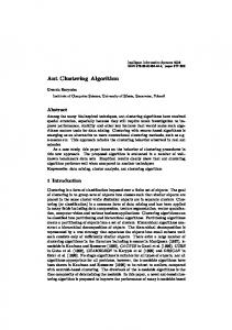
Figure 12 shows time-frequency analysis of r echo signals from a two-blade rotor helicopter. The window length is 64 time-frequency and the order interval 0.1.signals Figurefrom 12aa indicates algorithm Figure 12 shows analysis of risecho two-blade that rotor STFT helicopter. works The wellwindow only in the isbottom andorder the interval top signal analysis. Figure 12b,c show the length 64 and the is 0.1.time-frequency Figure 12a indicates that STFT algorithm works well only in the bottom and the top signal time-frequency analysis. Figure 12b,c show the results results when the order is not consistent. STFRFT performs better than STFT in both local signal when the order is not consistent. STFRFT analysis. performs better than the STFTrotation in both local signal detection detection and comprehensive frequency Finally, frequency of the and propeller comprehensive frequency analysis. Finally, the rotation frequency of the propeller blade in Figure 12d blade in Figure 12d is 35 revolutions per second, which agrees with the theoretical value of the is 35 revolutions per second, which agrees with the theoretical value of the helicopter model. Please helicopter model. Please refer to the markings of the time-frequency curve parameters in Figure 13 refer to the markings of the time-frequency curve parameters in Figure 13 for the computation of the for therotation computation of the rotation rateTcofrepresents the propeller, where, Tc represents a rotational period of rate of the propeller, where, a rotational period of the propeller, the rotation the propeller, the rotation frequency being thei.e., reciprocal of the period, i.e., 1/Tc. frequency being the reciprocal of the period, 1/Tc.
(a)
(b)
(c)
(d)
FigureFigure 12. Time-frequency analysis ofof helicopter signals.(a)(a)STFT STFT results; (b) STFRFT (p = 0.9) 12. Time-frequency analysis helicopter echo echo signals. results; (b) STFRFT (p = 0.9) results; (c) STFRFT (p = 1.1) results; (d) STFRFT results after comprehensive processing. results; (c) STFRFT (p = 1.1) results; (d) STFRFT results after comprehensive processing.
Sensors 2016, 16, 1559 Sensors2016, 2016,16, 16,1559 1559 Sensors Sensors 2016, 16, 1559
12 of 17 12ofof17 17 12 12 of 17
Doppler (Hz) Doppler (Hz)(Hz) Doppler
1000 1000 1000
Onecycle cycle One One cycle Tc Tc Rotation Rotation Tc rate=1/Tc Rotation rate=1/Tc rate=1/Tc
500 500 500 00 0 -500 -500 -500
Bladeno.1 no.1 Blade Blade no.1
-1000 -1000 00 -1000 0
0.01 0.01 0.01
Bladeno.2 no.2 Blade Blade no.2 0.02 0.02 Time (s) 0.02 Time (s) Time (s)
0.03 0.03 0.03
0.04 0.04 0.04
Figure13. 13.Diagram propellerparameters. parameters. Figure 13. Diagramof ofpropeller propeller parameters. Figure Figure 13. Diagram of propeller parameters.
4.3.Signals Signalsfrom fromthe theBird BirdTarget Target 4.3. 4.3. Signals from the Bird Target 4.3. Signals from the Bird Target Figure 14 14shows showsthe the bird target model [35],micro the micro micro Doppler echoof signal of which isis Figure shows the bird target model inin [35], the Doppler echo signal Figure bird target model in [35], the Doppler echo signal whichof iswhich analyzed Figure 14 shows the bird target model in [35], the micro Doppler echo signal of which is analyzed usingthe theproposed proposed technique. analyzed technique. using theusing proposed technique. analyzed using the proposed technique.
(a) (a) (a)
(b) (b) (b)
(c) (c) (c)
Figure14. 14.Micro MicroDoppler Dopplertime-frequency time-frequencyanalysis analysisofofflapping flappingwings. wings.(a) (a)Bird Birdtarget targetmodel; model;(b) (b)STFT; STFT; Figure Figure 14. (a) Bird Bird target target model; model; (b) (b) STFT; STFT; Figure 14. Micro Micro Doppler Doppler time-frequency time-frequency analysis analysis of of flapping flapping wings. wings. (a) (c) STFRFT. (c) STFRFT. (c) (c) STFRFT. STFRFT.
Supposingthe theradar radarwave wavelength lengthisis0.03 0.03m, m,the thetime timeof ofaccumulation accumulationisis10 10s,s,the thenumber numberof of Supposing Supposing the radar wavethe length is 0.03 m, the time of is lower 10 s, number of time of accumulation accumulation s, the the number of accumulated impulses is 8192, bird wing length is 1 m (both the upper and arms being 0.5 accumulated impulses is 8192, the bird wing length is 1 m (both the upper and lower arms being 0.5 accumulated impulses is 8192, 8192, thebird bird wing lengthis 1mm (both the upper and lower arms being impulses is the wing length 1shows (both upper and lower arms being 0.5 mlong), long),and andthe the flapping frequency Hz.Figure Figure 14isshows thethe processing results using STFT and m flapping frequency isis22Hz. 14 the processing results using STFT and 0.5 m long), the flapping frequency 2 Hz. Figure 1415 shows the processing results using STFT m long), andand the flapping frequency is differences, 2 is Hz. Figure 14 shows the processing results using STFT and STFRFT and, forbetter better revealing their Figure provides enlarged views ofthe the red box STFRFT and, for revealing their differences, Figure 15 provides enlarged views of red box and STFRFT and, for better revealing their differences, Figure 15 provides enlarged views of the STFRFT and, for better revealing their differences, Figure 15 provides enlarged views of the red box areas in Figure 14. It is apparent that STFRFT performs appreciably better than STFT areas in Figure 14. It is apparent that STFRFT performs appreciably better than STFT inin red box areas in Figure 14. It is apparent that STFRFT performs appreciably better than STFT in areas in Figure 14. It is apparent that STFRFT performs appreciably better than STFT in time-frequencyfocusing. focusing. time-frequency time-frequency time-frequency focusing. focusing.
(a) (a) (a)
(b) (b) (b)
Figure15. 15.Enlarged Enlargedviews viewsofofportions portionsofofFigure Figure14. 14.(a) (a)STFT; STFT;(b) (b)STFRFT. STFRFT. Figure Figure 15. 15. Enlarged views of of portions portions of of Figure Figure 14. 14. (a) (a) STFT; STFT; (b) (b) STFRFT. STFRFT. Figure Enlarged views
4.4.Actual ActualFan FanTarget TargetSignals Signals 4.4. 4.4. Actual Fan Target Signals 4.4. Actual Fan Target Signals To further further verify verify micro-Doppler micro-Doppler features features of of propeller propeller type type targets, targets, fan fan blades blades were were used used toto To Tofurther further verify micro-Doppler features of propeller type targets, fan were blades were used to simulate a helicopter propeller in an experiment. To verify micro-Doppler features of propeller type targets, fan blades used to simulate simulate a helicopter propeller in an experiment. a helicopter in an experiment. asimulate helicopter propeller propeller in an experiment.
Sensors 2016, 16, 1559
13 of 17
Sensors Sensors2016, 2016,16, 16,1559 1559
13 13ofof17 17
4.4.1. Dual-Blade Fan 4.4.1. 4.4.1.Dual-Blade Dual-BladeFan Fan Figure 16 shows a self-manufactured dual-blade fan, whose blades are 30 cm long and 3 cm wide. Figure 16 shows aaself-manufactured dual-blade fan, blades 30 long and cm Figure 16may shows self-manufactured fan,whose whose bladesare are 30cm cm long and33are cm The fan motor produce a rotation speeddual-blade up to 15 r/s. The parameters of the radar system wide. The fan motor may produce a rotation speed up to 15 r/s. The parameters of the radar system wide.inThe fan6.motor maysponges produceina Figure rotation up to 15 r/s. The parameters of the radar system given Table The blue 16speed are absorption materials. are aregiven givenininTable Table6.6.The Theblue bluesponges spongesininFigure Figure16 16are areabsorption absorptionmaterials. materials.
Figure 16. A dual-blade fan. Figure Figure16. 16.AAdual-blade dual-bladefan. fan. Table 6. Main parameters of radar system. Table Table6.6.Main Mainparameters parametersofofradar radarsystem. system.
Parameter Parameter Parameter Frequency Frequency Frequency Baseband sampling rate Baseband sampling Baseband sampling rate rate Accumulation Accumulation time Accumulation time time Target Target Target
ValueValue Value 3 GHz (continuous 3 GHz (continuous wave) 3 GHz (continuous wave) wave) 20 kHz 20 kHz 20 kHz 0.15 s0.15 0.15ss Fan Fan Fan
Figure 17a,b and STFRFT respectively, STFT having aa Figure17a,b 17a,bshow showthe theprocessing processingresult resultusing usingSFFT SFFT Figure show the processing result using SFFT and and STFRFT STFRFT respectively, respectively, STFT STFT having having window length of 16 and STFRFT a window length of 32, with the rest of the parameters being the ofof 32,32, with thethe rest of of thethe parameters being the awindow windowlength lengthofof1616and andSTFRFT STFRFTa awindow windowlength length with rest parameters being same for both techniques. It is obvious from Figure 17a,b that STFRFT fares better in resolving same for both techniques. It is obvious from Figure 17a,b that STFRFT fares better in resolving the same for both techniques. It is obvious from Figure 17a,b that STFRFT fares better in resolving time-frequency than STFT, as reveals more time-frequency component signals. time-frequencythan thanSTFT, STFT,as asitititreveals revealsmore moretime-frequency time-frequencycomponent componentsignals. signals. time-frequency 2000 2000 Doppler frequency(Hz) Doppler frequency(Hz)
Doppler frequency(Hz) Doppler frequency(Hz)
2000 2000 1000 1000 0
0
-1000 -1000 -2000 -2000 0
0
0.05 0.05
time(s) time(s)
(a) (a)
0.1 0.1
0.15 0.15
1000 1000 0
0
-1000 -1000 -2000 -2000 0
0
0.05 0.05
time(s) time(s)
0.1 0.1
0.15 0.15
(b) (b)
Figure 17. analysis ofoftwo techniques. (a) STFT; (b) STFRFT. Figure17. 17.Comparative Comparativeanalysis analysisof twotechniques. techniques.(a) (a)STFT; STFT;(b) (b)STFRFT. STFRFT. Figure Comparative two
4.4.2. Three-Blade Fan 4.4.2.Three-Blade Three-BladeFan Fan 4.4.2. The experiment fan shown in Figure 18, and the system parameters are ininTable 6.6.The Theexperiment experimentfan fanisisis shown Figure system parameters aregiven given Table The The shown in in Figure 18,18, andand thethe system parameters are given in Table 6. The fan fan shown in Figure 18 is an industrial ox horn fan (rotation speed: 18–23 r/s); Figure 19 shows the fan shown in Figure 18 is an industrial ox horn fan (rotation speed: 18–23 r/s); Figure 19 shows the shown in Figure 18 is an industrial ox horn fan (rotation speed: 18–23 r/s); Figure 19 shows the STFRFT STFRFT time-frequency analysis result ofofthis fan, the window length being 256. STFRFT time-frequency analysis result this fan, the window length being 256. time-frequency analysis result of this fan, the window length being 256. Unlike Figures 12d and 17b, the increased number of blades makes impossible totodetermine UnlikeFigures Figures12d 12dand and17b, 17b,the theincreased increasednumber numberof ofblades bladesmakes makesitititimpossible impossibleto determine Unlike determine clearly the number of time-frequency curves from Figure 19. Alternately, a blade (shown ininred clearly the number of time-frequency curves from Figure 19. Alternately, a blade (shown red clearly the number of time-frequency curves from Figure 19. Alternately, a blade (shown in red boxes) boxes) boxes)on onFigure Figure19 19isisfound foundtotohave havetime-frequency time-frequencyfeatures featuresnot notidentical identicaltotoother otherblades. blades.This Thisisis on Figure 19 is found to have time-frequency features not identical to other blades. This is because the because becausethe thetarget targetattitude attitudehas hassome someinfluence influenceon onthe theblades, blades,which whichare arelocated locateddifferently differentlyininspace. space. target attitude has some influence on the blades, which are located differently in space. Consequently, Consequently, the micro-Doppler signals generated by different blades may have Consequently, the micro-Doppler signals generated by different blades may haveslight slightdifferences. differences. Thus, Thus,we wecan canuse usethe thesame sameblade bladerecurring recurringcycle cycletotoestimate estimateblade bladenumber. number.
Sensors 2016, 16, 1559
14 of 17
the micro-Doppler signals generated by different blades may have slight differences. Thus, we can use Sensors 2016, 16, 1559 1559 14 of of 17 17 the same blade recurring cycle to estimate blade number. Sensors 2016, 16, 14
Figure 18. 18. Three-blade Three-blade fan. fan. Figure Figure 18. Three-blade fan.
Doppler Dopplerfrequency(Hz) frequency(Hz)
2000 2000
1000 1000
00
-1000 -1000
-2000 -2000 00
0.05 0.05
time (s) (s) time
0.1 0.1
0.15 0.15
Figure 19. STFRFT STFRFT time-frequency time-frequency analysis. analysis. Figure19. Figure19. STFRFT time-frequency analysis.
The period of the time-frequency spectrum on on Figure 19 (in (in red) red) cannot cannot be be extracted extracted directly. The time-frequency spectrum on Figure Figure 19 extracted directly. directly. Hence, technique of image registration is used to extract the spectrum of this period. Image Hence, image registration is used extract the spectrum of this period. Image registration Hence, technique techniqueofof image registration is to used to extract the spectrum of this period. Image registration detectsimages and selects selects images with with identical scenes by selecting selecting proper subtemplate and detects and selects with identical scenes by selecting a proper subtemplate and moving it over registration detects and images identical scenes by aa proper subtemplate and moving it over the entire image. When the subtemplate coincides with a portion of the entire image, the entire image. When the subtemplate coincides with a portion of the entire image, the correlation moving it over the entire image. When the subtemplate coincides with a portion of the entire image, the correlation correlation coefficient reaches maximum and the period of the the same image could could becorrelation extracted. coefficient reaches maximum and the period of thethe same image could be extracted. The the coefficient reaches maximum and period of same image be extracted. The correlation correlation coefficient is: is: coefficient is: coefficient The E ( S1 S2 ) ρ = √ E((D S11(SSS122)))D(S2 ) E S M N D((SS11))D D((SS122 )) ∑ D ∑ s1 (m,n)s2 (m,n) MN m M =1N Nn=1 = s M 11M N 2 s (m, n1 ) s M(mN, n)2 1 s11()][ m,MN n) s22∑(m∑ , n)s2 (m,n)] [ MN (16) ∑ ∑ s1 (m,n MN m=11 nn11 MN m=1 nm m =1 n =1 M MN N M N 11 M ∑N ∑s22 s(1m(m,n 11 )M N s22 (m, n)] )s2 (m,n )][ (16) [[ s s111 (m,, nn)][ s22 (m, n)] (16) m =1 n = = MN MN Mmm11 Nnn11 MN m 1 n 1 M MN N m 1 n 1 [M M ∑ NN∑ s21 (m,n)][ ∑ ∑ s22 (m,n)] = = = = ss ((mm,, nn))ss ((mm,, nn)) m 1n 1
m11 nn11 m 1N M N M 22 11 m11 nn11 m
11
m 1n 1 22
where ρ is the correlation coefficient, S the template image, and S2 the entire image, and ( M, N ) the M N N M template image size. [[ ss ((m )][ ss2222 ((m )] m,, nn)][ m,, nn)] m11image m nn11 Figure 20 shows the correlation coefficient after registration on Figure 19 by Equation (16). With a template sizecorrelation of 5 × 5, it is found that Sblade is 0.0463 theentire rotation frequency where is the the coefficient, therecurring templatecycle image, and sSSand the image, and S11 the where is correlation coefficient, template image, and 22 the entire image, and is 22 per second. After processing the frequency value using the method reported in [2], the number of M ,, N N )) the template template image image size. size. ((M availablethe blades is estimated at three, consistent with the actual number. For comprehensive validation, Figure 20 20 shows shows the the correlation correlation coefficient coefficient after image image registration registration on on Figure 19 19 by by Equation Equation Figure the same experiment and method were applied onafter different blades, all resultingFigure in accurate estimation (16). With With aa template template size size of of 55 ×× 5, 5, it it is is found found that that blade blade recurring recurring cycle cycle is is 0.0463 0.0463 ss and and the the rotation rotation (16). of the blade number n. frequency is 22 per second. After processing the frequency value using the method reported in [2], [2], frequency is 22 per second. After processing the frequency value using the method reported in the number number of of available available blades blades is is estimated estimated at at three, three, consistent consistent with with the the actual actual number. number. For For the comprehensive validation, the same experiment and method were applied on different blades, all comprehensive validation, the same experiment and method were applied on different blades, all resulting in accurate estimation of the blade number n. resulting in accurate estimation of the blade number n.
Sensors 2016, 16, 1559 Sensors 2016, 16, 1559
15 of 17 15 of 17
Correlation coefficient
1 X: 0.0463 Y: 0.9863
0.9 0.8 0.7 0.6 0.5
0
0.05
time (s)
0.1
0.15
Figure Figure 20. 20. Estimated rotation rotation period period of of blades. blades.
5. Discussion 5. Discussion This paper paperproposes proposesa aSTFRF-based STFRF-basedtime-frequency time-frequency algorithm. This new algorithm increases This algorithm. This new algorithm increases the the signal length the analysis window and enhances target and frequency To signal length in theinanalysis window and enhances target SNR andSNR frequency resolution.resolution. To overcome overcome the heavy computation load associated with the conventional STFRF, paper proposes the heavy computation load associated with the conventional STFRF, this paperthis proposes an order an order prediction technique makes of signal continuity subsisting within a short time, prediction technique that makes that use of signaluse continuity subsisting within a short time, thus improving thusadaptability improvingofthe of the proposed technique. analysis of a rotor the theadaptability proposed technique. The analysis of a rotorThe helicopter indicates that,helicopter when the indicates that, when the number of blades is two, the blade number can be accurately determined number of blades is two, the blade number can be accurately determined from STFRFT time-frequency from STFRFT image.exceeds When the number of blades exceeds two, it would difficult image. When time-frequency the number of blades two, it would be difficult to determine the be number of to determine the number of blades directly from STFRFT time-frequency image, duetime-frequency to the presence blades directly from STFRFT time-frequency image, due to the presence of multiple of multiple time-frequency spectrumusing lines. image This paper suggests using image registration technique spectrum lines. This paper suggests registration technique to estimate the recurrence to estimate the recurrence period a sameofblade wellSTFRFT as the domain numbertime-frequency of blades fromspectrum. STFRFT period of a same blade as well as theof number bladesasfrom domain time-frequency spectrum. Experiment data validated the effectiveness of this technique in Experiment data validated the effectiveness of this technique in determining the period and number of determining the period and number of blades of a multiple-blade target. blades of a multiple-blade target. This paper paperproposes proposesand and verifies characteristics and advantages of STFRFT. However, it This verifies thethe characteristics and advantages of STFRFT. However, it should should be noted that STFRFT transformation requires that the windowed signals must be noted that STFRFT transformation requires that the windowed signals must approximately be LFM approximately be LFM In practical radar applications, the signal time might be signals. In practical radarsignals. applications, the signal sampling time might be shortsampling and the window length short and the window length might be STFRFT’s limited and this wouldFor reduce advantages. For might be limited and this would reduce advantages. futureSTFRFT's work, a super-resolution future work, a super-resolution spectrum estimation technique may be investigated to further spectrum estimation technique may be investigated to further improve STFRFT’s performance in improve STFRFT's performance in time-frequency analysis. time-frequency analysis. Acknowledgments: This work was supported by Joint Doctorial Fund Project from the Ministry of Education, Acknowledgments: This work was supported by Joint Doctorial Fund Project from the Ministry of Education, PRC (2013142012007) (2013142012007) and and research research funds fundsof ofNorth NorthUniversity Universityof ofChina. China. PRC Author Contributions: Contributions:Cunsuo CunsuoPang Pangprovided provided insights formulating ideas, performed the simulations, Author insights in in formulating thethe ideas, performed the simulations, and analyzed the simulation results.results. Yan Han and Huiling Hou provided some insights motivation and basic idea and analyzed the simulation Yan Han and Huiling Hou provided someon insights on motivation and in introduction. ShenghengShengheng Liu and Nan carefully therevised paper. the paper. basic idea in introduction. LiuZhang and Nan Zhangrevised carefully Conflicts of Interest: The authors declare no conflict of interest. Conflicts of Interest: The authors declare no conflict of interest.
References References 1. 1. 2. 2.
3. 3. 4. 4.
5.
Chen, V.C.; Li, F.; Ho, S.S. Analysis of micro-Doppler signatures. IEEE Proc. Radar Sonar Navig. 2003, 150, Chen, V.C.; Li, F.; Ho, S.S. Analysis of micro-Doppler signatures. IEEE Proc. Radar Sonar Navig. 2003, 150, 271–276. [CrossRef] 271–276. Thayaparan, T.; Abrol, S.; Riseborough, E.; Stankovic, L.J.; Lamothe, D.; Duff, G. Analysis of radar Thayaparan, T.; Abrol, S.; Riseborough, E.; Stankovic, L.J.; Lamothe, D.; Duff, G. Analysis of radar micro-Doppler signatures from experimental helicopter and human data. IEEE Proc. Radar Sonar Navig. 2007, micro-Doppler signatures from experimental helicopter and human data. IEEE Proc. Radar Sonar Navig. 1, 289–299. [CrossRef] 2007, 1, 289–299. Ding, Y.; Tang, J. Micro-Doppler trajectory estimation of pedestrians using continuous-wave radar. IEEE Trans. Ding, Y.; Tang, J. Micro-Doppler trajectory estimation of pedestrians using continuous-wave radar. IEEE Geosci. Remote Sens. 2014, 52, 5807–5819. [CrossRef] Trans. Geosci. Remote Sens. 2014, 52, 5807–5819. Zhang, W.; Li, K.; Jiang, W. Parameter estimation of radar targets with macro-motion and micro-motion Zhang, W.; Li, K.; Jiang, W. Parameter estimation of radar targets with macro-motion and micro-motion based on circular correlation coefficients. IEEE Signal Process. Lett. 2015, 22, 633–637. [CrossRef] based on circular correlation coefficients. IEEE Signal Process. Lett. 2015, 22, 633–637. Lie-Svendsen, O.; Olsen, K.E.; Johnsen, T. Measurements and signal processing of helicopter micro-Doppler signatures. In Proceedings of the 11th European Radar Conference (EuRAD), Rome, Italy, 18 December 2014; pp. 121–124.
Sensors 2016, 16, 1559
5.
6. 7. 8. 9. 10. 11. 12. 13. 14.
15.
16.
17. 18.
19. 20. 21. 22. 23. 24.
25. 26. 27. 28.
16 of 17
Lie-Svendsen, O.; Olsen, K.E.; Johnsen, T. Measurements and signal processing of helicopter micro-Doppler signatures. In Proceedings of the 11th European Radar Conference (EuRAD), Rome, Italy, 8–10 October 2014; pp. 121–124. Baczyk, ˛ M.K.; Samczynski, ´ P.; Kulpa, K. Micro-Doppler signatures of helicopters in multistatic passive radars. IEEE Proc. Radar Sonar Navig. 2015, 9, 1276–1283. [CrossRef] Yang, B.; He, F.; Jin, J.; Xiong, H.; Xu, G. DOA estimation for attitude determination on communication satellites. Chin. J. Aeronaut. 2014, 27, 670–677. [CrossRef] Liu, Z.; Wang, Z.; Xu, M. Cubature Information SMC-PHD for Multi-Target Tracking. Sensors 2016, 16, 653. [CrossRef] [PubMed] Tahmoush, D. Review of micro-Doppler signatures. IEEE Proc. Radar Sonar Navig. 2015, 9, 1140–1146. [CrossRef] Fairchild, D.P.; Narayanan, R.M. Multistatic micro-doppler radar for determining target orientation and activity classification. IEEE Trans. Aerosp. Electron. Syst. 2016, 52, 512–521. [CrossRef] Stankovi´c, L.; Stankovi´c, S.; Thayaparan, T. Separation and reconstruction of the rigid body and micro-doppler signal in ISAR Part I-Theory. IEEE Proc. Radar Sonar Navig. 2015, 9, 1147–1154. [CrossRef] Satzoda, R.K.; Suchitra, S.; Srikanthan, T. Parallelizing the Hough transform computation. IEEE Signal Process. Lett. 2008, 15, 297–300. [CrossRef] Thayaparan, T.; Stankovic, L.; Dakovic, M.; Popovic, V. Micro-Doppler parameter estimation from a fraction of the period. IEEE Signal Process. Lett. 2010, 4, 201–212. [CrossRef] Suresh, P.; Thayaparan, T.; Obulesu, T.; Venkataramaniah, K. Extracting micro-Doppler radar signatures from rotating targets using Fourier-Bessel transform and time-frequency analysis. IEEE Trans. Geosci. Remote Sens. 2014, 52, 3204–3210. [CrossRef] Zhang, R.; Li, G.; Clemente, C.; Varshney, P.K. Helicopter classification via period estimation and time-frequency masks. In Proceedings of the IEEE 6th International Workshop on Computational Advances in Multi-Sensor Adaptive Processing (CAMSAP), Saint Martin, France, 13–16 December 2015; pp. 61–64. Du, L.; Li, L.; Wang, B.; Xiao, J. Micro-Doppler Feature Extraction Based on Time-Frequency Spectrogram for Ground Moving Targets Classification With Low-Resolution Radar. IEEE Sens. J. 2016, 16, 3756–3763. [CrossRef] Jokanovi´c, B.; Amin, M.; Dogaru, T. Time-frequency signal representations using interpolations in joint-variable domains. IEEE Trans. Geosci. Remote Sens. 2015, 12, 204–208. [CrossRef] Chen, X.; Guan, J.; Huang, Y.; Liu, N.; He, Y. Radon-linear canonical ambiguity function-based detection and estimation method for marine target with micro motion. IEEE Trans. Geosci. Remote Sens. 2015, 53, 2225–2240. [CrossRef] Ozaktas, H.M.; Zalevsky, Z.; Kutay, M.A. The Fractional Fourier Transform; Wiley: New York, NY, USA, 2001. Tao, R.; Deng, B.; Zhang, W.Q.; Wang, Y. Sampling and sampling rate conversion of band limited signals in the fractional Fourier transform domain. IEEE Trans Signal Process. 2008, 56, 158–171. [CrossRef] Suo, P.C.; Tao, S.; Tao, R.; Nan, Z. Detection of high-speed and accelerated target based on the linear frequency modulation radar. IEEE Radar Sonar Navig. 2014, 8, 37–47. [CrossRef] Pang, C.S.; Hou, H.L.; Han, Y. Acceleration target detection based on LFM radar. Optik-Int. J. Light Electron Opt. 2014, 125, 5708–5714. [CrossRef] Hou, H.; Pang, C.; Guo, H.; Qu, X.; Han, Y. Study on high-speed and multi-target detection algorithm based on STFT and FRFT combination. Optik-Int. J. Light Electron Opt. 2016, 127, 713–717. [CrossRef] Luo, Y.; Liu, H.W.; Gu, F.F.; Zhang, Q. Ground moving targets imaging via compressed sensing based on discrete FrFT. In Proceedings of the IEEE International Conference on Signal Processing, Communications and Computing (ICSPCC), Guilin, China, 19–22 September 2015; pp. 1–5. Qian, W.; Fei, Y.; Yi, Z.; En, C. Gabor Wigner Transform based on fractional Fourier transform for low signal to noise ratio signal detection. In Proceedings of the OCEANS, Shanghai, China, 10–13 April 2016; pp. 1–4. Tao, R.; Li, Y.L.; Wang, Y. Short-time fractional Fourier transform and its applications. IEEE Trans. Signal Process. 2010, 58, 2568–2580. [CrossRef] Chen, X.; Guan, J.; Bao, Z.; He, Y. Detection and extraction of target with micro motion in spiky sea clutter via short-time fractional Fourier transform. IEEE Trans. Geosci. Remote Sens. 2014, 52, 1002–1018. [CrossRef] Eldar, Y.C.; Sidorenko, P.; Mixon, D.G.; Barel, S.; Cohen, O. Sparse phase retrieval from short-time Fourier measurements. IEEE Signal Process. Lett. 2015, 22, 638–642. [CrossRef]
Sensors 2016, 16, 1559
29. 30.
31. 32. 33. 34. 35.
17 of 17
Catherall, A.T.; Williams, D.P. High resolution spectrograms using a component optimized short-term fractional Fourier transform. Signal Process. 2010, 90, 1591–1596. [CrossRef] Bai, X.; Tao, R.; Wang, Z.; Wang, Y. ISAR imaging of a ship target based on parameter estimation of multicomponent quadratic frequency-modulated signals. IEEE Trans. Geosci. Remote Sens. 2014, 52, 1418–1429. [CrossRef] Griffin, D.; Lim, J. Signal estimation from modified short-time Fourier transform. IEEE Trans. Acoust. Speech Signal Process. 1984, 32, 236–243. [CrossRef] Giv, H.H. Directional short-time Fourier transform. J. Math. Anal. Appl. 2013, 399, 100–107. [CrossRef] Pang, C.S. An accelerating target detection algorithm based on DPT and fractional Fourier transform. Acta Electron. Sin. 2012, 40, 184–188. Kim, B.; Kong, S.H.; Kim, S. Low computational enhancement of STFT-based parameter estimation. IEEE J. Sel. Top. Signal Process. 2015, 9, 1610–1619. [CrossRef] Chen, V.C. The micro-Doppler Effect in Radar; Artech House: Boston, MA, USA, 2011. © 2016 by the authors; licensee MDPI, Basel, Switzerland. This article is an open access article distributed under the terms and conditions of the Creative Commons Attribution (CC-BY) license (http://creativecommons.org/licenses/by/4.0/).