blog classification and temperature prediction suggest that the ... The authors gratefully acknowledge support from the NSF through ..... Tech. Rep., Carnegie Mellon University, Aug. 1994. [11] L. A. Adamic and N. Glance, âThe political ...
DISTRIBUTED ALGORITHM FOR GRAPH SIGNAL INPAINTING Siheng Chen1,2 , Aliaksei Sandryhaila3 , Jelena Kovaˇcevi´c1,2,4 1
Dept. of ECE, 2 Center for Bioimage Informatics, 3 HP Vertica, 4 Dept. of BME, Carnegie Mellon University, Pittsburgh, PA, USA ABSTRACT
We present a distributed and decentralized algorithm for graph signal inpainting. The previous work obtained a closed-form solution with matrix inversion. In this paper, we ease the computation by using a distributed algorithm, which solves graph signal inpainting by restricting each node to communicate only with its local nodes. We show that the solution of the distributed algorithm converges to the closed-form solution with the corresponding convergence speed. Experiments on online blog classification and temperature prediction suggest that the convergence speed of the proposed distributed algorithm is competitive with that of the centralized algorithm, especially when a graph tends to be regular. Since a distributed algorithm does not require to collect data to a center, it is more practical and efficient. Index Terms— Signal processing on graphs, graph signal inpainting, distributed and decentralized computing 1. INTRODUCTION The problem of collecting and analyzing data obtained from or represented by networks has been receiving increasing interest due to the abundance of such data in various research fields. Recently, a theoretical framework called graph signal processing has emerged as a new approach to analyze signals with irregular structure [1, 2, 3]. Its key idea is to represent the structure of a signal with a graph by associating signal coefficients with graph nodes and analyzing graph signals by using appropriately defined signal processing techniques, such as Fourier transform, filtering, and wavelets. One task of analyzing data represented by graphs is to reconstruct or estimate graph signal coefficients that are missing, unmeasurable, or corrupted, called graph signal inpainting [4, 5, 6]. The approach via minimizing graph total variation provide a closed-form solution, which involves matrix inversion [7, 8]. To solve this, we propose a distributed and decentralized algortithm for graph signal inpainting that can be computed locally in the vertex domain without transmitting signal coefficients to a computing center. We show that the The authors gratefully acknowledge support from the NSF through awards 1130616 and 1017278, and CMU Carnegie Institute of Technology Infrastructure Award. This paper is an extended version.
solution of the algorithm converges to the closed-form solution with certain convergence speed. We finally compare the convergence performance with a conventional centralized algorithm in the tasks of online blog classification and temperature prediction. 2. DISCRETE SIGNAL PROCESSING ON GRAPHS In this section, we briefly review relevant concepts of discrete signal processing on graphs; a thorough introduction can be found in [1, 2]. Discrete signal processing on graphs is a theoretical framework that generalizes classical discrete signal processing from regular domains, such as lines and rectangular lattices, to irregular structures that are commonly described by graphs. Graph shift. DSPG deals about signals with complex, irregular structure that is represented by a graph G = (V, A), N ×N where V = {vi }N i=1 is the set of nodes and A ∈ C is a graph shift, or a weighted adjacency matrix. Each Ai,j contains the edge weight between the ith node and the jth node, which characterizes their relation. For example, the edge weight can quantify similarities and dependencies between nodes, or indicate communication patterns in networks. Graph signals. Using this graph, we refer to a signal with structure as a graph signal, which is defined as a map that assigns a signal coefficient xn ∈ C to the graph node vn , and write it in a vector form, � �T x = x1 , x2 , · · · , xN ∈ CN . Graph total variation. A concept often used in signal processing is that of smoothness. Smoothness of graph signals is expressed by a graph total variation function 1 A x , (1) TVA (x) = x − |λmax (A)| 1 where λmax (A) denotes the eigenvalue of A with the largest magnitude. For notational simplicity, assume that the graph shift A has been normalized to satisfy λmax (A) = 1. Note that when the graph shift A is the cyclic permutation matrix, it represents time-series signals, and (1) reduces to the same definition from classical signal processing. Often, the quadratic form of graph total variation is used instead [9], 2
S2 (x) = ||x − A x||2 .
(2)
We use the quadratic form of the graph total variation for two reasons. First, it is computationally easier to optimize than the `1 -norm based graph total variation in (1). Second, the `1 -norm based graph total variation, which penalizes less transient changes than the quadratic form, is good at separating smooth from non-smooth parts of graph signals; the goal here, however, is to force graph signals at each node to be smooth. 3. GRAPH SIGNAL INPAINTING VIA TOTAL VARIATION MINIMIZATION
3.2. Graph total variation minimization When the uncorrupted part of the signal needs to be preserved intact, we solve (4) directly for � = 0, b x
=
arg min S2 (x), x
(7)
xM = tM .
subject to
Since we focus on minimizing the quadratic form of graph total variation, (7) is called the minimization approach. By e in a block form as writing A " # e MM A e MU A e= A e UM A e UU , A
In this section, we briefly review previous work on graph signal inpainting, which lays a foundation for the distributed algorithms shown later. For more details on graph signal inpainting, see [7, 8, 9]. We consider a corrupted graph signal measurement � � � � tM wM = t=x+w = x+ , (3) tU wU
the closed-form solution is as follows [7]:
where x is a true graph signal, tM ∈ CM is the uncorrupted part of the signal and tU ∈ CN −M is the corrupted part, wM is noise with small variance, and wU is corruption. The goal of graph signal inpainting is to recover x from t by removing the corruption w. We assume that the true signal x in (3) has low variation with respect to the underlying graph, represented by the graph shift A; we recover the true graph signal by solving the following minimization problem.
The closed-form solutions of both the regularization approach and the minimization approach requires inverting a matrix. When we deal with large graphs, that computation is expensive. To solve this, we propose the corresponding distributed and decentralized algorithms for both regularization and minimization approaches and show the properties of convergence.
e −1 e b U = −A x U U AU M tM .
(8)
4. DISTRIBUTED GRAPH TOTAL MINIMIZATION FOR SIGNAL INPAINTING
4.1. Distributed graph total variation regularization b x subject to
=
arg min S2 (x),
(4a)
||wM ||22 ≤ �2 ,
(4b)
t = x + w.
(4c)
x
The condition (4b) controls the noise level of wM . 3.1. Graph total variation regularization
We propose the following algorithm as a distributed and decentralized counterpart of (5): Algorithm 1. (Distributed graph total variation regularization) e with α such that ||h(A)||2 < 1. Let h(A) = I −α(ΦM + λA), Set the intial conditions as k = 0, x(0) = 0, and do the following two steps iteratively:
To get a closed-form solution, the graph signal inpainting (4) can be formulated as an unconstrained problem as, b = arg min ||xM − tM ||22 + λ S2 (x), x x
(5)
where the tuning parameter λ controls the trade-off between the two parts of the objective function. Since the quadratic form of graph total variation is a regularization term, (5) is called the regularization approach. The closed-form solution is as follows [7]: �
e b = ΦM + λ A x
�−1
x(k+1)
←
h(A)x(k) + αb t,
k
←
k + 1,
until convergence. In (9), the value of the nth node is updated as x(k+1) n
=
(6)
� � � � I 0 b t e = (I − A)∗ (I − A), where ΦM = MM ,t= M ,A 0 0 0 and ∗ denotes the Hermitian transpose.
N X
b h(A)n,m x(k) m + αtn
m=1
= b t,
(9)
N X
((1 − αλ) I −αΦM
m=1
b +α(A∗ + A − A∗ A))n,m x(k) m + α tn , P where (A∗ A)n,m = i A∗i,n Ai,m . When the value of An,m , or A∗n,m , is nonzero, there exists an edge between the nth and
mth node; when the value of (A∗ A)n,m is nonzero, there is at least one node connecting the nth and mth node. We thus see that when the geodesic distance between the nth node and the mth node is more than 2, h(A)n,m is always zero; in other words, the value of each node is updated by weighting the values of its local neighbors and adding a pre-stored constant. This algorithm can be computed by each node without transmitting signal coefficients to a computing center, which is distributed and decentralized. The following theorem provide theoretical insight into Algorithm 1.
4.2. Distributed graph total variation minimization We propose the following algorithm as a distributed and decentralized counterpart of (7). Algorithm 2. (Distributed graph total variation minimization) e with α such that ||g(A)U U ||2 < 1. Set the Let g(A) = I −αA, (0) (0) intial conditions as k = 0, xM = tM , xU = 0, and do the following three steps iteratively
x
Theorem 1. Let k → ∞, where k is the iteration number. The solution of Algorithm 1 converges to (6) with the convergence error decreasing as O(||h(A)||k2 ).
xM
(k)
←
tM ,
(k+1)
←
g(A)x(k) ,
k
←
k + 1,
(11)
until convergence.
Proof. From (9), we have
In (11), the value of the nth node is updated as x(k)
= (a)
=
(b)
=
h(A)x(k−1) + αb t � � h(A) h(A)x(k−2) + αb t + αb t α
k−1 X
x(k+1) n
h(A) t,
(10)
(a)
=
α
+∞ X
h(A)ib t
i=0 (b)
=
α(I −h(A))−1b t
(c)
=
e −1b α(α(ΦM + λA)) t
(d)
e −1b (ΦM + λA) t,
=
where (a) follows (10), (b) follows the matrix inversion property, (c) follows the definition of h(A) and (d) cancels α. Denote x = limk→+∞ x(k) , we have ||x
(k)
− x||2
g(A)n,m x(k) m
(a)
=
||α
+∞ X
ib
h(A) t||2
i=k
=
k
||(h(A)) α
+∞ X
h(A)ib t||2
i=0 (b)
=
(c)
≤
||(h(A))k x||2 ||(h(A)||k2 ||x||2 ,
where (a) and (b) follow (10), and (c) follows the definition of spectral norm. By rearranging the terms, we finally obtain ||x(k) − x||2 ||x||2
=
N X
((1 − α) I +α(A∗ + A − A∗ A))n,m x(k) m ,
m=1
where (a) follows (9) by setting k to k − 1 and (b) comes from the induction. We then have
k→+∞
N X m=1
ib
i=0
lim x(k)
=
≤
||(h(A)||k2 .
P ∗ where (A∗ A)n,m = i Ai,n Ai,m . Similarly h(A) in (9), when the geodesic distance between the nth node and the mth node is more than 2, g(A)n,m is always zero. This algorithm is also distributed and decentralized. The following theorem shows the sufficient condition for ||g(A)U U ||2 ≤ 1, which provides a way of choosing α. e Then, Theorem 2. Let 0 < α ≤ 2/λmax (A). ||g(A)U U ||2 ≤ 1. e is real and symmetric, we decompose it as Proof. Since A e A
=
U Λ U∗ ,
(12)
where U is an unitary matrix and Λ are a diagonal matrix whose diagonal elements are are the corresponding eigenvalues, denoted as λi ; moreover, λ1 ≥ λ2 ≥ . . . ≥ λN ≥ 0. e we have Since 0 < α ≤ 2/λmax (A), e ≥ −1. 1 ≥ 1 − αλi ≥ 1 − 2λi /λmax (A) We then bound the spectral norm of g(A)U U as (a)
||g(A)U U ||2
≤ (b)
||g(A)||2
=
e 2 || I −αA||
(c)
=
|| I −α U Λ U∗ ||2
(d)
|| U(I −αΛ) U∗ ||2
=
(e)
=
(f )
max |1 − αλi | ≤ 1, i
(13)
where (a) comes from the property of spectral norm, (b) follows the definition of g(A), (c) follows (12), (d) comes from the unitary property of U, (e) comes from the definition of spectral norm and (f ) follows (13).
where (a) and (b) follow (14), and (c) follows the definition of spectral norm. We finally obtain (k)
||xU − xU ||2 ||xU ||2
≤
||(g(A)U U )||k2 .
The following theorem provides a theoretical insight into Algorithm 2. Theorem 3. Let k → ∞, where k is the iteration number. The solution of Algorithm 2 converges to (8) with the convergence error decreasing as O(||g(A)U U ||k2 ). Proof. From (11), we split x based on uncorrupted indices and corrupted indices as "
(k+1)
xM (k+1) xU
# =
� g(A)MM g(A)U M
g(A)MU g(A)U U
� " (k) # xM (k) . xU
We focus on the uncorrupted indices of x and obtain (k+1)
xU
(k)
(k)
=
g(A)U M xM + g(A)U U xU
(a)
k X
=
(0)
(g(A)U U )i g(A)U M xM
i=0
=
k X
(g(A)U U )i g(A)U M tM ,
(14)
i=0
where (a) comes from the induction and (b) comes from the initialization of setting the corrupted part to be zero. We then obtain (k+1)
lim xU
k→+∞
=
lim
k→+∞
k X
(g(A)U U )i g(A)U M tM
i=0
(a)
=
(IU U −g(A)U U )−1 g(A)U M tM
(b)
=
e U U )−1 (−αA e U M )tM (αA
=
e UU A e U M tM , −A
−1
where (a) comes from the property of the matrix inversion and (b) follows the definition of g(A). (k) Denote xU = limk→+∞ xU , (k)
||xU − xU ||2
(a)
=
= (b)
=
(c)
≤
The algorithms to solve graph total variation regularization as in (5) and graph total variation minimization as in (7) are distributed and decentralized because each node can be updated individually in each iteration without transmitting signal coefficients to a computing center, this, however, requires an infinite number steps to converge. Since both (5) and (7) are quadratic problems, one alternative is conjugate gradient descent [10], which produces the exact solution after a finite number of iterations. Conjugate gradient descent, however, is a centralized method and requires more storage space. Although it converges faster than the distributed algorithm, it takes more computation in each iteration. We compare the two versions in the following section. 5. EXPERIMENTAL RESULTS
(0)
+(g(A)U U )k+1 xU (b)
4.3. Discussion
We now apply the proposed algorithms to the classification of online blogs and temperature inpainting. We compare the proposed algorithms with centralized method, conjugate gradient descent. Note that in both cases, we build directed graph with asymmetric graph shift, which cannot be handled by graph Laplacian-based methods [5, 6]. As mentioned in 4.3, the conjugate gradient descent use all the information, and the distributed methods only use the local information. Therefore, the the conjugate gradient descent should converge faster, but the distributed methods compute separately at each node, which saves the storage space. Here the experiments verify that the convergence speed of the proposed distributed method catches up with that of the conjugate gradient descent when the graph trends to be regular. 5.1. Classification of online blogs
We consider the problem of classifying N = 1224 online political blogs as either conservative or liberal [11]. We represent conservative labels as +1 and liberal ones as −1. The blogs +∞ are represented by a graph in which nodes represent blogs, X || (g(A)U U )i g(A)U M tM ||2 and directed graph edges correspond to hyperlink references i=k between blogs. For a node vn its outgoing edges have weights +∞ X 1/ deg(vn ), where deg(vn ) is the out-degree of vn (the num||(g(A)U U )k (g(A)U U )i g(A)U M tM ||2ber of outgoing edges). i=0 We randomly labeled 1% of blogs and applied the graph k total variation minimization to estimate the labels for remain||(g(A)U U ) xU ||2 ing nodes. Estimated labels were thresholded around zero, so that positive values were set to +1 and negative to −1. We ||(g(A)U U )||k2 ||xU ||2 ,
e Note that the graph shift represents set α to be 1/λmax (A). a scale-free graph whose degree distribution follows a power law. In Figures 1 and 2, we compare the convergence performance between the proposed algorithm and the conjugate gradient descent. The convergence error is defined as e(k) =
||x(k) − x||22 , ||x||2
where x(k) is the result in the kth iteration and x is the closedform solution. We see that conjugate gradient descent converges much faster than the proposed distributed algorithm. The reason is that some popular blogs connect most of the nodes and some other blogs are isolated from the others, which leads to a large ||g(A)||2 . From Theorem 2, we know that a large ||g(A)||2 causes a slow convergence. 1.6
Convergence error
Ai,j = Pi,j /
P
i
Pi,j , where N 2 di,j Pi,j = exp − P , i,j di,j
where di,j is the geodesic distances between the ith and the jth weather stations. Note that the graph shift represents a direct graph where each node has the same number of neighbors, which is more regular than the graph shift in Section 5.1. For each of 365 recording, we randomly corrupted 50% of measurements and applied the graph total variation minimization to estimate those measurements. We set α to be e 1/λmax (A). In Figures 3 and 4, we compare the convergence performance between the proposed algorithm and conjugate gradient descent. We see that the proposed algorithm converges by using almost the same iterations with conjugate gradient descent. The reason is that we build a regular graph that each node has the same degree, which leads to a small ||g(A)||2 . From Theorem 2, we know that a small ||g(A)||2 causes a fast convergence. From these two experiments, we Convergence error
1.4 1
1.2 1
0.8
Theoretical
0.8
0.6
0.6 0.4 0.2 0 0
Proposed method 0.4
Conjugate gradient descent 100
200
300
400
Proposed method Conjugate gradient descent
0.2 500
Iterations
600
700
800
900
1000 0 0
Fig. 1: Convergence error as a function of the iteration number for online blog classification. 1
Theoretical
Accuracy
10
20
30
40
50
Iterations
60
70
80
90
100
Fig. 3: Convergence error as a function of the iteration number for temperature inpainting.
0.9
Conjugate gradient descent 0.8
4000
Proposed method
Mean square error
3500
0.7
3000 0.6
2500
Conjugate gradient descent 0.5 0.4 0
2000 1500 100
200
300
400
500
Iterations
600
700
800
900
1000 1000 500
Fig. 2: Classification accuracy as a function of the iteration number for online blog classification. 5.2. Temperature inpainting We consider 150 weather stations in United States that record their local temperatures [1, 12]. Each weather station has 365 records, in total of 54750 measurements. The graph representing these weather stations is obtained by measuring the geodesic distance between each pair of weather stations. The nodes are represented by an 8-nearest neighbor graph, in which nodes represent weather stations, and each node is connected to eight other nodes that represent the closest weather stations. The graph shift A is constructed as
0 0
Proposed method 10
20
30
40
50
Iterations
60
70
80
90
100
Fig. 4: Mean square error as a function of the iteration number for temperature inpainting. conclude that on more regular graphs, the convergence speed of the proposed distributed and decentralized algorithm is almost as fast as the centralized method. Since a distributed algorithm does not require to collect data to a center, it is more practical and efficient. 6. CONCLUSION In this paper, we presented distributed and decentralized algorithms for graph signal inpainting. The algorithms solve
graph signal inpainting by restricting each node to communicate only with its neighbors. We showed that the solution of the distributed algorithm converges to the closed-form solution with the theoretical convergence speed. Experiments on online blog classification and the temperature prediction suggest that the convergence speed of the proposed distributed algorithm is competitive with that of the centralized algorithm, especially when a graph tends to be regular. Since a distributed algorithm does not require to collect data to a center, it is more practical and efficient. 7. REFERENCES [1] A. Sandryhaila and J. M. F. Moura, “Discrete signal processing on graphs,” IEEE Trans. Signal Process., vol. 61, no. 7, pp. 1644–1656, 2013. [2] A. Sandryhaila and J. M. F. Moura, “Discrete signal processing on graphs: Frequency analysis,” IEEE Trans. Signal Process., vol. 62, no. 12, pp. 3042–3054, 2014. [3] D. I. Shuman, S. K. Narang, P. Frossard, A. Ortega, and P. Vandergheynst, “The emerging field of signal processing on graphs: Extending high-dimensional data analysis to networks and other irregular domains,” IEEE Signal Process. Mag., vol. 30, pp. 83–98, 2013. [4] A. Elmoataz, Olivier Lezoray, and S. Bougleux, “Nonlocal discrete regularization on weighted graphs: A framework for image and manifold processing,” IEEE Trans. Image Process., vol. 17, no. 7, pp. 1047–1060, 2008. [5] X. Zhu, Z. Ghahramani, and J. Lafferty, “Semisupervised learning using gaussian fields and harmonic functions,” in Proc. ICML, 2003, pp. 912–919. [6] M. Belkin, P. Niyogi, and P. Sindhwani, “Manifold regularization: A geometric framework for learning from labeled and unlabeled examples.,” J. Machine Learn. Research, vol. 7, pp. 2399–2434, 2006. [7] S. Chen, A. Sandryhaila, G. Lederman, Z. Wang, J. M. F. Moura, P. Rizzo, J. Bielak, J. H. Garrett, and J. Kovaˇcevi´c, “Signal inpainting on graphs via total variation minimization,” in Proc. IEEE Int. Conf. Acoust., Speech Signal Process., Florence, Italy, May 2014. [8] S. Chen, A. Sandryhaila, J. M. F. Moura, and J. Kovaˇcevi´c, “Signal denoising on graphs via graph filtering,” in Proc. IEEE Glob. Conf. Signal Information Process., Atlanta, GA, Dec. 2014. [9] S. Chen, A. Sandryhaila, J. M. F. Moura, and J. Kovaˇcevi´c, “Signal recovery on graphs,” IEEE Trans. Signal Process., 2014, Submitted.
[10] Jonathan Richard Shewchuk, “An introduction to the conjugate gradient method without the agonizing pain,” Tech. Rep., Carnegie Mellon University, Aug. 1994. [11] L. A. Adamic and N. Glance, “The political blogosphere and the 2004 u.s. election: Divided they blog,” in Proc. LinkKDD, 2005, pp. 36–43. [12] NCDC NOAA 1981-2010 climate normals, ,” 2011, ncdc.noaa.gov/oa/climate/normals/usnormals.html.