i = 1 : N stands for the enumeration i = 1, 2, ... N; the superscripts ·T and ·H stand for transpose and Hermitian ... In general, the channel matrix for Rician fading can be written as [1]: ... ios measured in [9] are reproduced in Table I. This table also.
This full text paper was peer reviewed at the direction of IEEE Communications Society subject matter experts for publication in the IEEE ICC 2011 proceedings
MIMO Zero-Forcing Detection Performance for Correlated and Estimated Rician Fading with Lognormal Azimuth Spread and K -Factor Constantin Siriteanu, Xiaonan Shi, Yoshikazu Miyanaga Graduate School of Information Science and Technology Hokkaido University, Sapporo 060-0814, Japan Abstract—For multiple-input multiple-output (MIMO) wireless communications systems, we propose a new zero-forcing (ZF) detection approach that explicitly accounts for instantaneous channel state information (ICSI) estimation error and spatial correlation. For this ZF approach we derive an average error probability (AEP) expression for transmit-correlated Rician fading. This AEP derivation exploits the effective signal-to-noise ratio that results by compounding ICSI estimation error and receiver noise and the approximation of the ensuing noncentralWishart distribution with a simpler central Wishart distribution. The derived AEP expression is then applied to evaluate MIMO ZF performance in Rayleigh and Rician fading for samples from recently-measured lognormal azimuth spread (AS) and Rician Kfactor distributions, for pilot-based ICSI estimation. Numerical results depict the dependence of the AEP averaged over the AS and K distributions on fading type, rank of the deterministic component of the channel matrix, and AS–K correlation, for realistic scenarios. Index Terms—Azimuth spread, correlation, K-factor, MIMO, Rician fading, zero-forcing detection.
I. INTRODUCTION A. Background Multiple-input multiple output (MIMO) concepts are promoted for next-generation wireless communications systems due to the capacity and symbol-detection performance gains promised by multi-antenna theory [1] [2]. However, these gains may not be always fully achievable in practice due to channel condition [3] (geometry; fading type, e.g., Rayleigh or Rician; fading parameters, e.g., azimuth spread (AS) and Rician K-factor) and transceiver impairments (instantaneous channel state information — ICSI — estimation error), as we attempt to show in this paper, for the low-complexity linear MIMO detection method known as zero-forcing (ZF). B. Previous Work ZF average bit-error rate expressions have been derived for M -QAM and M -PSK, transmit-correlated Rician fading, and perfectly-known ICSI in [4] [5] [6], by approximating the noncentral Wishart distribution of the matrix that enters the signal-to-noise ratio (SNR) expression of the ZF detector with a central Wishart distribution. For estimated ICSI, ZF closed-form average bit-error rate expressions for M -QAM and M -PSK and uncorrelated
Rayleigh fading appear in [7, Eqns. (20), (21)]. The disadvantages of the approach in [7] are that it employs two approximations and it requires knowledge of the mapping between the CSI estimation method and its error. The advantage is that the ICSI estimation error is compounded with the receiver noise into the effective (i.e., actual) symbol-detection noise, and the analysis exploits the resulting effective SNR. For estimated ICSI, an exact MIMO ZF detection performance analysis appears, also for uncorrelated Rayleigh fading, in [8]. As in [7], the ZF detection matrix is constructed from the ICSI estimate as if it were the true ICSI [8, Eqn. (11)]. However, only the ICSI estimation error due to nonintended streams is compounded with the receiver noise. Then, the effective signal-to-interference-plus-noise ratio is employed to derive closed-form average symbol-error rate expressions for M -PAM and QPSK. To the best of our knowledge, MIMO ZF has yet to be evaluated comprehensively based on average error probability (AEP) expression for practical correlated spatial channel models. Such models have recently become available from the European WINNER II project, which measured actual channels for a wide range of environments [9]. WINNER II has revealed preponderantly-Rician fading with scenariodependent AS and K lognormal distributions and correlations. We recently employed these models to evaluate SIMO performance based on AEP expression [10] and (generic and IEEE 802.11n) MIMO performance based on simulations [11] [12]. C. Contributions and Approach For transmit-correlated Rician fading and SNR-dependent ICSI estimation error model, a new ZF detection approach is proposed and systematically analyzed (for M -PSK), based on the effective SNR obtained by compounding the ICSI estimation error on all streams with the receiver noise. This analysis yields a simpler and more widely-applicable AEP expression than those from [4] [7] [8]. This AEP expression is used to evaluate ZF symboldetection performance for fading models and AS and K distributions and correlation that characterize actual scenarios as described in [9]. The AEP expression is first computed for samples from the lognormal AS and K distributions with scenario-dependent mean, variance, and correlation from [9, Table 4-5]. Then, the AEP is numerically averaged over these
978-1-61284-231-8/11/$26.00 ©2011 IEEE
This full text paper was peer reviewed at the direction of IEEE Communications Society subject matter experts for publication in the IEEE ICC 2011 proceedings
AS and K samples. The new AEP expression can reduce simulation effort substantially. D. Notation Scalars, vectors, and matrices are represented in lowercase italics, boldface lowercase, and boldface uppercase, respectively, e.g., x, x, and X; x ∼ Nc (x, X) indicates that x is a complex-valued circularly-symmetric random vector [1, p. 39] of multivariate Gaussian distribution with mean x and covariance X; ψ ∼ N (0, 1) indicates that scalar ψ is a real-valued random variable of Gaussian distribution with zero-mean and unit variance; subscripts ·d and ·r identify, respectively, the deterministic (mean) and random components of a scalar or vector; index ·n indicates a normalized variable; i = 1 : N stands for the enumeration i = 1, 2, . . . N ; the superscripts ·T and ·H stand for transpose and Hermitian (complex-conjugate) transpose; [·]i and [·]i,j indicate the ith and i, jth element of a vector and a matrix, respectively; E{·} denotes statistical average. E. Paper Organization Section II introduces statistical models for transmitted signal, channel fading, AS, and K. Section III describes the new ZF detection approach for imperfect ICSI and shows the AEP derivation. Section IV presents relevant numerical results. II. S YSTEM M ODEL A. Signal and Channel Fading Models We consider a single-user MIMO wireless communication system over a frequency-flat Rician fading channel. Let us assume that there are NT and NR antenna elements at the transmitter and receiver, respectively, with NT ≤ NR . Letting x = [x1 x2 · · · xNT ]T denote the NT -dimensional vector with the transmitted symbols (M -PSK modulation, E{xxH } = INT ), the NR -dimensional vector with the received signals can be represented as [1, p. 63]: � Es Hx + n, (1) r= NT where Es /NT is the energy transmitted per symbol, H is the NR × NT complex-valued channel matrix whose elements are assumed to have unit variance, and n is temporallyand spatially-white, circularly-symmetric, zero-mean, complex Gaussian, i.e., n ∼ Nc (0, N0 I) [1]. Let us denote the deterministic (i.e., mean) and random components of H as Hd and Hr , respectively, i.e., H = Hd + Hr . When Hd is non-zero and the elements of Hr are complex-valued Gaussian random variables, | [H]i,j | has a Rician distribution, whereas for zero channel mean, | [H]i,j | has a Rayleigh distribution [2]. In general, the channel matrix for Rician fading can be written as [1]: � � K 1 Hd,n + Hr,n , (2) H = Hd + Hr = K +1 K +1 where Hd,n is the normalized deterministic component (mean) of H, i.e., with �Hd,n �2 = NT NR , and Hr,n is the normalized
random component of H, i.e., with E{| [Hr,n ]i,j |2 } = 1, ∀i = 1 : NR , j = 1 : NT . Since E{�Hr,n �2 } = NT NR , the channel matrix it is properly normalized, i.e., E{�H�2 } = NT NR [13]. Thus, the power ratio of the deterministic and the random components of H is �Hd �2 = E{�Hr �2 }
K 2 K+1 �Hd,n � 1 2 K+1 E{�Hr,n � }
= K,
(3)
which is known as the Rician K-factor [1]. Channel and antenna geometry determine the rank of Hd,n and, thus, MIMO system performance. For transmitter– receiver distance much larger than antenna interelement distance (such as in typical sub/urban and rural scenarios) this rank is likely low or unitary [1, p. 41]. Then, performance has been found to degrade with increasing K [1, p. 79] [4, Fig. 4]. For transmitter–receiver distance similar to antenna interelement distance (such as in indoor scenarios) this rank is likely high or even NT . Then, performance has been found to improve with increasing K [1, p. 79] [4, Fig. 4]. Let us assume that there is transmit correlation but no receive correlation, as in the downlink from a high base-station antenna to a mobile station immersed in a rich-scattering environment. Then, we can use the MIMO correlation model 1/2 Hr,n = Hw RT , where RT is the NT × NT transmit correlation matrix, and Hw has independent and identically distributed circularly-symmetric, zero-mean, complex Gaussian, unit-variance elements [1]. The rows of Hr,n are mutually independent whereas each of them has correlation matrix RT . B. Statistical Models for AS and K The AS (which approximates the root mean square of the power azimuth spectrum — PAS) and the K-factor determine the mean and variance of the channel fading gains (i.e., the channel matrix elements) and, thus, performance. Multiantenna performance assessments have typically assigned arbitrary or extreme values to K and spatial correlation [1] [2]. However, comprehensive measurements undertaken by the European WINNER II project [9] indicate that AS and K can both be modeled as lognormal random variables with scenariodependent means and variances. For example, for the indoor office/residential scenario denoted as A1 in [9], the AS (in degrees) and K have been modeled as: AS = 100.31 χ+1.64 , K = 100.1 (6 ψ+7) ,
χ ∼ N (0, 1),
(4)
ψ ∼ N (0, 1).
(5)
The AS and K distributions for the other line-of-sight scenarios measured in [9] are reproduced in Table I. This table also shows the AS–K correlation, i.e., the correlation coefficient of χ from (4) and ψ from (5). Scenario A1 experiences the strongest (negative) such correlation. The Laplacian PAS, which has been found to model accurately received power in actual channels [9], is expressed in terms of the AS in [14, Eqns. (4.2), p. 136]. Then, AS affects the elements of RT as shown in [14, Eqns. (4.3)-(4.4), pp. 136-137].
This full text paper was peer reviewed at the direction of IEEE Communications Society subject matter experts for publication in the IEEE ICC 2011 proceedings
TABLE I BASE - STATION AS AND K STATISTICS [9, TABLE 4-5] Scenario A1: indoor office/residential B1: typical urban microcell B3: large indoor hall C1: suburban C2: typical urban macrocell D1: rural macrocell D2a: rural, high-speed
AS [◦ ]
K
ρ
101.64+0.31χ 100.40+0.37χ 101.22+0.18χ 100.78+0.12χ 101.00+0.25χ 100.78+0.21χ 100.70+0.31χ
100.1(7+6ψ) 100.1(9+6ψ) 100.1(2+3ψ) 100.1(9+7ψ) 100.1(7+3ψ) 100.1(7+6ψ) 100.1(7+6ψ)
−0.6 −0.3 +0.2 +0.2 +0.1 +0.0 +0.0
III. MIMO ZF D ETECTION A PPROACH AND A NALYSIS A. ZF Detection for Perfect ICSI Assuming perfectly-known H, ZF detection for the received-signal from (1) means estimating the symbol transmitted through the kth antenna (i.e., xk ) by mapping the kth element of vector � � NT � H �−1 H NT � H �−1 H H H H H H r=x+ H n, (6) Es Es into the closest modulation constellation symbol (i.e., slicing). Note that, although there is no interference among the transmitted symbols in the ideal ZF detector, the symboldetection noises are correlated across the data streams. Thus, ZF detection is suboptimal, but has been widely studied because it yields low-complexity MIMO receivers [1, p. 153]. B. Conventional ZF Detection Approach for Estimated ICSI Assuming availability of an estimate G of H, ZF detection is typically undertaken by simply replacing H with G in (6), i.e., with [7] [8]: � NT � H �−1 H G G G r. (7) Es This approach is easy to implement but can be difficult to analyze. A ZF detection approach that can be analyzed more easily and that also better accounts for ICSI estimation accuracy is proposed next, based on our work for SIMO systems [15]. C. Distribution of Channel Given ICSI Estimate Let us assume that the channel matrix H and its estimate G are jointly Gaussian, as is the case for the popular ICSI estimation methods using PSAM and interpolation [15]. Let H H us denote by hH , with mean hH d , and g , with mean gd , corresponding rows from H and G. Then, the mean and covariance of h given g (both NT × 1) are [16, p. 562]: hm Re
= E{h|g} = E{h} + Rhg R−1 g (g − E{g}), H
= E{(h − hm )(h − hm ) |g} = Rh −
(8)
Rhg R−1 (9), g Rgh
D. New ZF Detection Approach for Estimated ICSI Substituting (10) into (1) recasts the received signal vector as follows: � � Es Es Hm x + He x + n, (11) r= NT N � � T �� ν
where ν comprises channel estimation error and actual noise and is, therefore, denoted effective noise [7]. Note that the new noise vector ν is zero-mean, complex-valued, Gaussiandistributed with correlation matrix:
Es H ν ν tr(Re ) + N0 INT . (12) E{ν } = NT Let us assume that beside G, the above covariance matrices are also known. This latter assumption is supported by the fact that the channel statistics fluctuate much more slowly than the channel gains [9] and, thus, can be estimated accurately for low per-symbol complexity [14] [15]. For ICSI estimation methods that employ pilot symbols and interpolation these covariance matrices can be computed as shown in [14] [18]. Then, in the new signal model (11), matrix Hm is known. Therefore, instead of conventional ZF detection as in (7) we can use the following new approach: � � �−1 H �−1 H NT � H NT � H Hm Hm Hm Hm Hm r = x + Hm ν . (13) Es Es Note that a comparison of the ZF detection approaches from (13) and (7) is beyond the scope of this work, although it is currently under investigation. Based on our previous investigations of similar approaches for SIMO, we anticipate that the new detector will yield better performance than the conventional one in highly-correlated channels, i.e., for predominantly-low AS [14, Fig. 3.13, p. 99]. Now, for the kth stream of the detector from (13), the instantaneous SNR can be expressed as [1] [4] [7] γk =
�k Γ , −1 ] [(HH m Hm ) k,k
(14)
� k is given by where Γ �k = Γ
Es NT
E{|[νν ]k |2 }
=
Es NT
Es NT tr(Re )
+ N0
.
(15)
E. ZF Detection AEP Derivation
Thus, given G, the channel matrix can be written as H = Hm + He ,
described by (9). Note that Hm is the MMSE estimate of H given G [17, p. 203] [8, Appendix 1]. Finally, Hm and the required covariance matrices can be computed for various ICSI estimation methods as in [14] [18].
(10)
where Hm has rows given by the vectors hH m described by (8), and He has rows whose distribution is Nc (0, Re ) and
For Rician fading the NT × NT matrix HH m Hm has a noncentral Wishart distribution that has been approximated with a central Wishart distribution [4]. Then, the symboldetection SNR for the kth data stream from (14) has a
This full text paper was peer reviewed at the direction of IEEE Communications Society subject matter experts for publication in the IEEE ICC 2011 proceedings
Gamma distribution [19, p. 103] described by shape parameter α = NR − NT + 1 and scale parameter β = Γk [4], where �k Γ Γk = � −1 � , Σ m k,k
(16) −1
with [4, Section 3]
10
=
1 H H Hd + Rm . NR d
(17)
Above, Rm is the covariance matrix of hm , which, based on (8), can be written as Rm = Rhg R−1 g Rgh . Hereafter, we discard the stream index k from our notation, for simplicity. Since γ from (14) is Gamma distributed with the parameters mentioned above, its probability density function (p.d.f.) is [4, Eqn. (4)]: p(γ) =
NR −NT
−γ/Γ
e 1 γ , (NR − NT )! ΓNR −NT +1
γ ≥ 0,
(18)
1 . (19) Γ Given the symbol-detection SNR γ, the M -PSK error probability can be written as [2, Eqn. (8.22)] �
MM−1 π π sin2 M 1 dθ. (20) exp −γ Pe (γ) = π 0 sin2 θ −(NR −NT +1)
,
−3
10
20
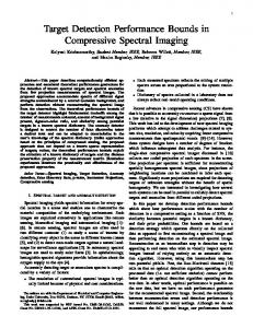
Rayleigh, Analysis Rayleigh, Simulation Rice, Analysis, K = 7 dB Rice, Simulation, K = 7 dB 22
24
26
28
30
32
34
36
38
40
Fig. 1. AEP from (22) and AER from simulation for ZF MIMO detection. Settings: perfectly known ICSI, QPSK modulation, NT = NR = 4, rank(Hd ) = 1, AS = 56.75◦ .
s