On Interleaving in Timed Automata⋆ Ramzi Ben Salah Marius Bozga Oded Maler V ERIMAG, 2, av. de Vignate, 38610 Gieres, France
[email protected] [email protected] [email protected]
Abstract. We propose a remedy to that part of the state-explosion problem for timed automata which is due to interleaving of actions. We prove the following quite surprising result: the union of all zones reached by different interleavings of the same set of transitions is convex. Consequently we can improve the standard reachability computation for timed automata by merging such zones whenever they are encountered. Since passage of time distributes over union, we can continue the successor computation from the new zone and eliminate completely the explosion due to interleaving.
1 Introduction Exploring the state space of timed automata [AD94] is a fundamental activity with numerous potential applications in circuit timing analysis, scheduling, verification of real-time software, performance analysis, etc. It is, however, a very difficult problem still waiting for a performance breakthrough despite efforts invested during the last 15 years. We hope that the results of this paper will advance us in this respect. Partial-order methods have been widely reported in the discrete verification literature. They focus on that part of the state-explosion problem posed by the interleaving semantics, as illustrated by the example of Figure 1 where we see two automata and their asynchronous composition. Actions a and b are mutually independent and hence, in the product automaton, state 11 can be reached via two paths1 that commute in a “diamond”. For certain simple reachability properties that do not mention paths and intermediate states, it is sufficient to explore only one of those paths. However, if additional non-commuting transitions are possible from the intermediate states, or if the properties are more sequential and less invariant under path permutations, the situation is more involved and has been a subject of numerous publications. This is not the topic of the present paper. In the analysis of timed automata, diamonds pose additional problems. Due to the clock variables, paths that seem to commute on the transition diagram do not necessarily converge to the same extended state which includes also the clock values. Consider the timed automata appearing in Figure 2 together with their composition. In each automaton the transition from 0 to 1 resets the respective clock. The standard reachability computation algorithm for timed automata computes a discrete directed graph, the ⋆
1
This is a slightly revised version of the CONCUR’06 paper, with additional references to related work which were brought to our attention after the submission of the final manuscript. In general, n! paths when there are n transitions.
0
0
a
00
b 10
1
01
1
11
Fig. 1. Two automata with independent action a and b, and their composition.
nodes of which are “symbolic states” of the form (q, Z) where q is a discrete state and Z is a zone, a convex set of clock valuations satisfying some conjunction of inequalities. Apply this algorithm to the automaton we obtain two zones associated with state 11, one in which x ≤ y (because in all runs along this path x is reset after y) and the other with y ≤ x. So here, in a situation where untimed reachability will converge to single state, timed reachability will generate several symbolic states from which the computation can be continued, leading very quickly to explosion. Roughly speaking, while the ordinary explosion associated with a product of n automata, each with m states will lead in the worst case to O(mn ) states, the additional splitting due to interleaving may result in O(nmn ) states, a fact that prevents verification of systems of modest size.2 In this paper we propose a solution to this problem, which is based on a new surprising3 result which shows that the set of all points in the clock space reached by runs consisting of interleaving of the same set of actions is convex. Since evolution distributes over union, zones that have been reached through different paths in the transition graph can be merged during reachability computation, thus eliminating the interleaving explosion. The rest of the paper is organized as follows. In Section 2 we give the definition of timed automata and their interaction. In Section 3 we prove our main result which is used in Section 4 to define a modified reachability algorithm whose superiority is experimentally confirmed. In Section 5 we discuss the applicability of the results to various forms of interaction, and conclude in Section 6 with a discussion of related work, in particular the idea of local time scales.
2 Timed Automata We consider a composition A1 ||A2 || · · · ||An of timed automata. Interaction can be defined using two types of mechanisms, the first one is by synchronized transitions and the other one, which is more expressive and useful, is by shared variables. To simplify the 2
3
Note that if we can push the size limit of timed verification toward non-trivial systems, the rest of the battle against explosion can continue from there using abstraction-based methods like the ones we have recently proposed [BBM03,BBM06]. What is surprising is the fact that this simple fact has not become part of the explicit collective knowledge of those working in the domain, the authors included.
0
00
0
x := 0
y := 0
a
b
y := 0
x := 0
10 1
00
01
x := 0
10
y := 0
01
1 y := 0
x := 0
11
y := 0
11 0 ≤ y ≤ x
x := 0
11 0 ≤ x ≤ y
Fig. 2. Two timed automata, their composition and an example of reachability computation.
presentation we will use the former to present our result and discuss later its extension to state-based synchronization. For the same pedagogical reasons, we make additional simplifying assumptions concerning the form of invariants and guards, but the results extend naturally to any conjunction of timed inequalities. As for non-convex (disjunctive) conditions allowed by the original definition of timed automata, we have found no use of them in more than 10 years experience in the domain.4 We also do not pay much attention to the distinction between strict and non strict inequalities which are irrelevant to convexity. Definition 1 (Timed Automaton). A timed automaton is A = (Σ, Q, C, I, ∆) where Σ is a finite set of transition labels, Q is a finite set of states, C is a finite set of clocks, I is the staying condition (invariant), assigning to every q ∈ Q a conjunction Iq of inequalities of the form c ≤ u, for some clock c and integer u, and ∆ is a transition relation consisting of elements of the form (q, g, a, r, q ′ ) where q and q ′ are states, a ∈ Σ is a transition label, g (the transition guard) is a conjunction of formulae of the form (c ≥ l) for some clock c and integer l and r ⊆ C is a set of clocks to be reset by the transition. We assume one transition labelled a for every a ∈ Σ. A clock valuation is a function v : C → R≥0 and a configuration of the automaton is a pair (q, v) consisting of a discrete state (location) and a clock valuation. We use r also to denote the reset function on clock valuation that sets the clock in r to zero and leaves the other intact. We use v + d to denote the clock valuation obtained from v by adding d to all clock values. A step of the automaton is one of the following: a
– A discrete step: (q, v) −→ (q ′ , v ′ ), for some transition (q, g, a, r, q ′ ) ∈ ∆ such that v satisfies g and v ′ = r(v). 4
The tendency to look for results proved for the “most general” definition, inherited uncritically from mathematics, can be sometimes very counter-productive in domains which are still evolving. Perhaps this could be one of the reasons for the sterility of certain branches of theoretical computer science.
d
– A time step: (q, v) −→ (q, v + d) for some d ∈ R≥0 such that v + d satisfies Iq . A compound step is a time step (possibly of a zero duration) followed by a discrete step: d,a
d
a
(q, v) −→ (q ′ , v ′ ) ≡ (q, v) −→ (q, v + d) −→ (q ′ , v ′ ). A run of the automaton starting from a configuration (q0 , v0 ) is a finite sequence of compound steps ending in a time step. ξ:
d1 ,a1
d2 ,a2
dk ,ak
d
∗ (q0 , v0 ) −→ (q1 , v1 ) −→ · · · −→ (qk , vk ) −→ (qk , vk + d∗ ).
ξ
We use also the notation (q, v) −→ (q ′ , v ′ ) for runs. We will define the interaction between the automata via a “distributed alphabet” Σ in the sense of the theory of traces [DR95]. For each automaton Ai , let Σ i be its local alphabet, that is the set of transition labels it uses. Our composition semantics requires that all Ai such that a ∈ Σ i should participate in an a-labelled global transition. Hence in any run of the global automaton an a-transition will be taken the same number of times in all Ai such that a ∈ Σ i . Definition 2 (Composition of Timed Automata). A composition of timed automata is A = A1 ||A2 || · · · ||An where each automaton is of the form Ai = (Σ i , Qi , C i , I i , ∆i ). The sets of states and clocks of the automata are mutually disjoint. The global automaton obtained from the composition is A = (Σ, Q, C, I, ∆) where Sn Sn n Q = Πi=1 Qi , C = i=1 C i and Σ = i=1 Σ i . We write global states as q = (q 1 , . . . , q n ) ∈ Q and global clock valuations over C as v = (v 1 , . . . , v n ). The semantics of the composition is given in terms of global steps as follows: a
– A discrete step: (q, v) −→ (q′ , v′ ), such that for every i either a ∈ Σ i and a (q i , v i ) −→ (q ′i , v ′i ) is a step of Ai , or a 6∈ Σ i and (q ′i , v ′i ) = (q i , v i ). d – A Vntime step: (q, v) −→ (q, v + d) for some d ∈ R+ such that v + d satisfies i=1 Iqi .
Global compound steps and runs are defined similarly to their local counterparts. It is sometimes (and this time in particular) useful to speak of the projection of a global run on each automaton. The projection ξ i of a global run ξ is obtained from ξ in two stages. First we “hide” transitions in which Ai does not participate and collapse the time passages, that is apply successively the following transformation: d,a
d′ ,a′
(q, v) −→ (q′ , v′ ) −→ (q′′ , v′′ )
7−→
a,d+d′
(q, v) −→ (q′′ , v′′ )
whenever a′ 6∈ Σ i . After all such external transitions have been eliminated we project the run on the states and clocks of Ai . Finally let us define two additional notions. Two runs ξ, ξ ′ of A are qualitatively equivalent if they go through the same sequence of discrete transitions and differ only in timing. We denote this fact by ξ ≈ ξ ′ and write equivalence classes of ≈ by [ξ]. We say that ξ and ξ ′ are locally equivalent, denoted by ξ ∼ ξ ′ , if all their local projections are equivalent, that is, ξ i ≈ ξ ′i for every i. We denote equivalence classes of ∼ as hξi. Clearly, ≈ is stronger than ∼, and perhaps too strong. When ξ ∼ ξ ′ , both runs agree on the order of local transitions while ξ ≈ ξ ′ means that they agree also on their interleaving.
3 Main Result We can now formulate our main result. Theorem 1 (Convexity). Let Z be a convex timed polyhedron and let q and q′ be two global states of A. Let ξ be a run starting at q and ending in q′ . Then the set [ ξ′ {v′ : ∃v ∈ Z (q, v) −→ (q′ , v′ )} RZ,hξi ≡ ξ ′ ∈hξi
is convex. The proof is given via a characterization of the reachable clock valuations by a quantified formula consisting of conjunctions of inequalities over clock values and auxiliary variables. Since convex sets are closed under projection the result follows. For economy of notation we assume that ξ is such that each automaton Ai makes exactly k steps. The restriction of Ai to the states and transitions involved in the run is of the form depicted in Figure 3.
i q0 i I0
i , ai , ri g1 1 1
i q1 i I1
···
i qk−1 i Ik−1
i , ai , ri gk k k
i qk i Ik
Fig. 3. The part of Ai which participates in ξ i .
As a first step we extend the description of local runs to include the time stamps of the transitions: i ξ i : (q0i , v0i , ti0 ) → (q1i , v1i , ti1 ) → · · · → (qki , vki , tik ) → (qki , vk+1 , tik+1 ).
Each tij variable denotes the absolute time in which the corresponding transition has been taken. Every global run in hξi is completely characterized by the values tij and vji for i = 1..n and j = 0..k + 1. All those runs satisfy the natural local ordering among time stamps, i.e. tij ≤ tij+1 , while those that are also ≈-equivalent agree also on the ordering of time stamps of different automata, which characterize the particular interleaving (shuffle) of the local runs. We can now proceed to the logical characterization. We will use the following auxiliary notations and abbreviations: qj = (qj1 , . . . qjn ) for global states, vj = (vj1 , . . . vjn ), for global clock valuations, vi = {v0i , . . . , vki }, for the set of valuations appearing in a i local run ξ i and ti = {ti0 , . . . , tS local time stamps. The set of all values k } for the set ofS that characterize a run are v = i vi , and t = i ti . The predicates {Φij } characterize the clock values and time stamps in a valid step j of Ai . ∃d d = tij − tij−1 ∧ i i + d) ∧ Ij−1 (vj−1 i Φij (vj−1 , tij−1 , vji , tij ) ≡ i i g (v + d) ∧ ji j−1i i vj = rj (vj−1 + d)
This is nothing but a recapitulation of the definition of a compound step, namely that time passage does not violate the staying condition, the transition guard is satisfied and that a reset takes place. Note that this definition is invariant under a shift of global time, that is, Φij (v, t, v ′ , t′ ) is equivalent to Φij (v, t + d, v ′ , t′ + d) for every d. We can now define what constitutes a valid run of Ai in isolation, without taking into account synchronization constraints. We keep this definition shift-invariant as well and do not yet insist on the initial zone which is defined globally. Φi (ti , vi ) =
k ^
i Φij (vj−1 , tij−1 , vji , tij )
j=1
The predicate which defines what constitutes a valid global run is a conjunction of the conditions for local runs with additional conditions that take care of all the synchronization aspects, including the fact that all runs start and terminate simultaneously. For every a ∈ Σ let Sa = {(i, j) : aij = a} be the set of steps that synchronize on a. To force all a-transitions to take place at the same time we define the predicate ^ ′ tij = tij ′ . Ψa (t) ≡ (i,j),(i′ ,j ′ )∈Sa
The conditions for a valid global run starting at Z0 are then: 1 n 2 t0 = t0 = · · · = t 0 ∧ v0 ∈ Z0 ∧ V n Φ(t, v) = Vi=1 Φi (vi , ti ) ∧ Ψa (t) ∧ 1 a∈Σ 2 tk+1 = tk+1 = · · · = tnk+1 Note that the first and last conditions can be viewed as synchronization conditions for two additional fictitious transitions “start” and “end” in which all automata participate. This set is a convex subset of the space consisting of all valuations and time stamps in the run, and so is its projection on the last n dimensions which is the reachable set: RZ,hξi (vk+1 ) ≡ ∃t∃v1 , . . . , vk Φ(t, v1 , . . . vk , vk+1 ). ⊓ ⊔ Let us mention that the result extends naturally to arbitrary “linear” hybrid automata with convex guards and invariants.
4 Application to Reachability Computation 4.1 A Modified Algorithm We will now modify the standard reachability computation algorithm for timed automata to take advantage of this result. The idea is to generate symbolic states in a breadth-first manner and at each level merge those reached by the same set of compound
steps. To identify those we need to decorate symbolic states with (partially ordered) path information. A shuffle expression over Σ is α = α1 || . . . ||αn with αi ∈ (Σ i )∗ . Concatenation of a shuffle expression and a symbol a is defined as (α1 || . . . ||αn ) · a = (β 1 || . . . ||β n ) where β i = αi if a 6∈ Σ i and β i = αi · a otherwise. Reachability computation for timed automata [HNSY94] is based on zones (timed polyhedra) which are expressed as conjunctions of rectangular inequalities of the form c ≤ d or c ≥ d and diagonal inequalities of the form c − c′ ≤ d for clocks c, c′ and integer d. A symbolic state is a pair (q, Z) where Z is a zone. The a-successor of a symbolic state (q, Z) such that q admits an a transition is defined as d,a
Suca (q, Z) = {(q ′ , v ′ ) : ∃v ∈ Z ∃d ≥ 0 (q, v) −→ (q ′ , v ′ ). The computation (q ′ , Z ′ ) = Suca (q, Z) is done by first applying “time passage” to Z, intersecting the result with Iq and with the transition guard and then applying the corresponding reset. This computation costs O(n3 ) time for n clocks. Algorithm 1 performs this computation. At each iteration Waiting is a list of extended zones to be explored, all reached by the same number of transitions. We compute the successors of all those symbolic states and put them in a list New. The Merge procedure scans New and replaces every subset of symbolic states of the form {(q, Z1 , α), . . . , (q, Zm , α)} by a single state (q, Z, α) where Z is the convex hull of all these zones. From our result it follows that Z is exactly the union of the zones. Note that the path labels of a zone need not be kept after its successors have been computed. This also guarantees termination due to the finite number of zones. Algorithm 1 (New Reachability Algorithm) Explored:= New:=∅ Waiting:={(q0 , Z0 , ε||..||ε)} while Waiting6= ∅ do for each (q, Z, α) ∈ Waiting such that (q, Z) 6∈ Explored do for each a ∈ Σ do New :=New∪{(Suca (q, Z), α · a)} Explored := Explored ∪{(q, Z)} Waiting := Merge(New) return(Explored) 4.2 Experimental Results To confirm the complexity reduction empirically we have first tested a preliminary implementation of Algorithm 1 restricted to products of chain-like automata. Such automata are notorious for generating state explosion due to interleaving. We have considered two simple families of synthetic benchmarks shown in Figure 4. The first consists of parallel compositions of n independent reset sequences of length m each. The second class consists of parallel compositions of k independent synchronization chains, each
being a parallel composition of n synchronized sequences of length m. A synchronized sequence (Aij ) alternates between actions that synchronize with the left (ai,j ) and the right (ai+1,j ) neighbor while separating them by at least 4 time units.
q0ij aij /xij := 0
q0i τi /xi := 0
kni=1
kkj=1 kni=1
q1i τi /xi := 0
r0ij [xij ≥ 4] ai+1j q1ij aij /xij := 0
i qm
ij qm
Fig. 4. The structure of the synthetic benchmarks.
The experimental results obtained for the two benchmarks for different values of n, m and k are summarized in Table 1. Each entry in the table is of the form B/C where B is the number of symbolic states encountered in an ordinary breadth-first exploration, while C is the number of states explored by Algorithm 1. We limit ourselves to instances with less than 106 symbolic states, and use the ⊥ symbol to denote the fact that this limit has been reached. Let us note that we achieve an exponential reduction both for the interleaving of independent actions (reset sequences) and for strongly-synchronized actions (a single synchronization chain with k = 1). The reduction is clearly much more impressive in the synchronized case, where reductions based on partial order or symmetry [HBL+ 03] are not directly applicable. We have then implemented Algorithm 1 into the IF toolset [BGM02] and tested its performance on several publicly-available benchmarks. Table 2 compares the performance of the new algorithm on the Fisher mutual-exclusion protocol benchmark with other reported results. We compare with old Kronos results reported in [T98], Uppaal results reported in [U] and results obtained with IF without using the new algorithm. It is interesting to note that although our new algorithm performs much better than the standard Uppaal machinery, their performances are similar when the convex-hull approximation option of the latter is employed. Our result shows that this “approximation” can be easily made exact.
5 Generalizations and Limitations Let us discuss briefly the applicability of our result to more general modes of interaction between timed automata. A crucial condition for expressing synchronization constraints
n=2 n=4 n=6 Independent reset sequences m=1 5/4 65 / 16 1957 / 64 m=2 13 / 9 633 / 81 75973 / 729 m=3 25 / 16 2713 / 256 732529 / 4096 Synchronization chains k = 1 m=1 4/4 6/6 8/8 m=2 8/8 37 / 17 236 / 30 m=3 12 / 12 86 / 32 1441 / 72 Synchronization chains k = 3 m=1 2012 / 64 812375 / 216 ⊥ / 512 m=2 97142 / 512 ⊥ / 4913 ⊥ / 27000 m=3 745197 / 1728 ⊥ / 32768 ⊥ / 373248
n=8
n=10
109601 / 256 ⊥ / 1024 ⊥ / 6561 ⊥ / 59049 ⊥ / 65536 ⊥/⊥ 10 / 10 12 / 12 1600 / 47 10949 / 68 30841 / 140 660615 / 244 ⊥ / 1000 ⊥ / 103823 ⊥/⊥
⊥ / 1728 ⊥ / 314432 ⊥/⊥
Table 1. Experimental results on the synthetic acyclic benchmarks.
Size 2 3 4 5 6 7 8 9 10 11
Kronos Uppaal Uppaal-A IF IF-U -/-/0.01s -/0.00s 29/0.003s 18/0.002s -/-/0.03s -/0.01s 165/0.01s 53/0.01s 752/-/0.23s -/0.06s 1099/0.07s 164/0.03s 3552/-/5.09s -/0.29s 8453/1.07s 527/0.04s 16320/- -/310.97s -/1.34s 74939/21.06s 1726/0.20s 73620/- -/51598.17s -/5.89s 762429/595.75s 5693/1.75s ⊥/⊥ ⊥/⊥ -/25.83s ⊥/⊥ 18792/5.73s ⊥/⊥ ⊥/⊥ -/113.53s ⊥/⊥ 61883/28.42s ⊥/⊥ ⊥/⊥ -/498.88s ⊥/⊥ 202994/367.76s ⊥/⊥ ⊥/⊥ -/2525.31s ⊥/⊥ 662873/4489.23s
Table 2. Results on the Fisher protocol benchmark. The Uppaal-A column corresponds to results obtained using the convex-hull approximation, while the IF-U column represents our new algorithm. Table entries represent the number of symbolic states and computation time. The symbol “-” means “ not reported” (or “irrelevant” for the case of computation time on older computers) and ⊥ means “too big”.
in a conjunctive form is that in every abstract run, every transition admits a unique set of transitions with which it is has to synchronize. This condition is fulfilled by requiring that whenever an a-transition takes place, all automata having a in their alphabet must participate. If a transition could choose some subset of the other transitions to synchronize with, Φ may contain disjunctions that cannot be eliminated and the result no longer holds. State-based synchronization in which the state of one or more automata may appear in the invariants and transition guards of other automata is more general and has a more asymmetric flavor as one automaton may enable a transition in the other without being obliged to take a transition by itself. Suppose A1 can take a transition when A2 is in state q and consider an abstract run in which A1 takes this transition and A2 passes through q twice (see Figure 5). Let t be the time stamp of the A1 transition, and let [t1 , t2 ] and [t3 , t4 ] be the time intervals in which A2 stays in q. The synchronization condition in this case will be disjunctive: t ∈ [t1 , t2 ] ∨ t ∈ [t3 , t4 ]. If, however, the disabling of the A1 transition is always accompanied by an explicit transition in A1 the run that synchronizes with the first sojourn in q and the one synchronizing with the second one, are not qualitatively equivalent and the result is preserved. This property holds, for example, in the automata we use to model bi-bounded inertial delays [MP95] as well as in models derived from free-choice Petri nets. A1
A2
q
A′1
true
q
q
q
¬q
¬q
q
Fig. 5. Automata A1 ||A2 do not satisfy Theorem 1 while A′1 ||A2 do.
Another illuminating example which is particularly important for our motivating application domain (circuits) is the following: let Ax , Ay and Az be three Boolean automata modeling an AND gate z = x ∧ y and consider runs in which both x and y rise from 0 to 1 and consequently z rises as well. Denoting the respective time stamps by tx , ty and tz , the synchronization condition is of the form (tx ≤ ty = tz ) ∨ (ty ≤ tx = tz ) or equivalently tz = max{tx , ty }, which does not define a convex set. In order to apply Algorithm 1 correctly to systems admitting this type of synchronization we need to split every such transition to several copies, each with a unique synchronization context. Let us remark that when the local automata are acyclic and reverse-deterministic (no state is entered via two different sequences of transitions), all global symbolic states that
agree on the discrete state are reached via the same set of transitions. Hence our result can be exploited without decorating the states with path information.
6 Related Work and Discussion The application of partial-order techniques to timed systems has been subject to several publications [R94,RM94,YS97,DGKK98,BJJY98,M99,Z02,LNZ05,ZYN03]. Although our simple result is related to some of the work mentioned in the next paragraph, it has not been stated explicitly and, moreover, its exploitation by a breadth-first version of the standard timed-automaton reachability algorithm has never been considered. The algorithm of Rokicki [R94,RM94], using a variant of timed Petri nets is similar to ours by computing a zone which corresponds to the interleaving of independent transitions. This work which has been done in parallel with the development of the first verification tools for timed automata, uses another terminology and has not proliferated to the timed automaton culture. Two more recent efforts, which are more ambitious with respect to full-fledged partial-order reductions, are those of Zhao [Z02] and of Niebert et al. [ZYN03,LNZ05]. Both works use additional clocks in their algorithms and use zones over the extended clock space (“event zones” in the terminology of [ZYN03,LNZ05], “local successors” in the terminology of [Z02]) that represent all configurations reached by interleavings of independent actions. We use the auxiliary clocks only in the proof of convexity which can be deduced via their results. It is worth noting that our result does not require independence of actions. It would be interesting to compare the reductions provided by the two approaches in terms of scope and performance. An interesting idea which was first proposed in [BJJY98], inspired by distributed simulation, is to use local time scales, that is to compute successors for each automaton separately on its own clock subspace, and somehow combine these local zones upon synchronization. Although the idea is aesthetically pleasing, it suffers from several problems including the implicit global synchronization that takes place at time zero, and the fact that you need to augment each automaton with an additional clock that measures its corresponding total elapsed time. This idea, however, inspired our proof of convexity. We prove, nevertheless, a small result which indicates the circumstances under which local time scales can be effectively exploited. We present the result informally. Consider two automata A1 and A2 and a prefix of a global run that reaches a global state (q 1 , q 2 ), and in which each of the two has passed through a local state in which all its clocks were inactive.5 If no synchronized action has taken place since then, one can see that if q 1 → q ′1 and q 2 → q ′2 via synchronization-free local runs, then (q 1 , q 2 ) → (q ′1 , q ′2 ) in the product automaton. The reason is that because of the clock inactivity, each of the local runs can be “delayed” and every local state that can be reached at time t can be reached as well at any t′ ≥ t and hence any pair of local states can be made to be reached simultaneously. This implies that after such a “desynchronization” point, reachable sets can be computed separately for each automaton and be 5
A clock is inactive in a state if along any path starting in that state it will be reset before being tested. This fact has been used to reduce the dimension of reachability computation [DY96].
merged via intersection before the next synchronization. This observation can be useful for verifying products of automata that repeatedly go through such inactive states. As a final remark, let us note that reducing the number of zones by taking their convex hull has been considered in the past [DT98] but always as an over-approximation. We speculate that the reason for not discovering the result of the present paper is due to the fact that the systems studied were cyclic, in which the same discrete state could be reached by different paths, not all of which being permutations of the same set of transitions. That is why the possibility of exact convex hull escaped the attention. In general we think that looking at the structure of individual runs can give insights that are sometimes masked by focusing exclusively on the reachability graph representation. Acknowledgment This paper has benefitted from discussions with P. Niebert.
References [AD94]
R. Alur and D.L. Dill, A Theory of Timed Automata, Theoretical Computer Science 126, 183-235, 1994. [BJJY98] J. Bengtsson, B. Jonsson, J. Lilius and W. Yi, Partial Order Reductions for Timed Systems, CONCUR’98, 485-500, 1998. [BBM03] R. Ben Salah, M. Bozga and O. Maler, On Timing Analysis of Combinational Circuits, FORMATS’03, 204-219, 2003. [BBM06] R. Ben Salah, M. Bozga and O. Maler, Automatic Abstraction of Timed Components, submitted, 2006. [BGM02] M. Bozga, S. Graf and L. Mounier, IF-2.0: A Validation Environment for Component-Based Real-Time Systems, CAV’02, 343-348, 2002. [DGKK98] D. Dams, R. Gerth, B. Knaack and R. Kuiper, Partial-order Reduction Techniques for Real-time Model Checking, Formal Aspects of Computing 10, 469-482, 1998. [DT98] C. Daws and S. Tripakis, Model Checking of Real-Time Reachability Properties Using Abstractions, TACAS’98, 313-329, 1998. [DY96] C. Daws and S. Yovine, Reducing the Number of Clock Variables of Timed Automata, RTSS’96, 73-81, 1996. [DR95] V. Diekert and G. Rozenberg (Eds.), The Book of Traces, World Scientific, 1995. [HBL+ 03] M. Hendriks, G. Behrmann, K. Larsen, P. Niebert and F. Vaandrager, Adding Symmetry Reduction to Uppaal, FORMATS’03, 46-59, 2003. [HNSY94] T. Henzinger, X. Nicollin, J. Sifakis, and S. Yovine, Symbolic Model-checking for Real-time Systems, Information and Computation 111, 193-244, 1994. [LNZ05] D. Lugiez, P. Niebert and S. Zennou, A Partial Order Semantics Approach to the Clock Explosion Problem of Timed Automata, Theoretical Computer Science 345, 27-59, 2005. [MP95] O. Maler and A. Pnueli, Timing Analysis of Asynchronous Circuits using Timed Automata, CHARME’95, 189-205, 1995. [M99] M. Minea, Partial Order Reduction for Model Checking of Timed Automata, CONCUR’99, 431-446, 1999. [R94] T.G. Rokicki, Representing and Modeling Digital Circuits, PhD Thesis, Stanford University, 1994. [RM94] T. Rokicki and C.J. Myers, Automatic Verification of Timed Circuits, CAV’94, 468480, 1984. [T98] S. Tripakis, The Analysis of Timed Systems in Practice, PhD Thesis, Universit´e Joseph Fourier, Grenoble, 1998.
[U] [YS97] [ZYN03] [Z02]
Uppaal benchmarks: www.it.uu.se/research/group/darts/uppaal/benchmarks T. Yoneda and B.-H. Schlingloff, Efficient Verification of Parallel Real-Time Systems, Formal Methods in System Design 11, 187-215, 1997. S. Zennou, M. Yguel and P. Niebert, ELSE: A New Symbolic State Generator for Timed Automata, FORMATS’03, 273-280, 2003. J. Zhao, Partial Order Path Technique for Checking Parallel Timed Automata, FTRTFT’02, 417-432, 2002.