Ubiquitous Computing and Communication Journal
AIR TRAFFIC ENROUTE CONFLICT DETECTION USING ADAPTIVE RESONANCE THEORY MAP NEURAL NETWORKS (ART1) 1
2
Krishan Kumar1 Invertis Institute of Management Studies, Bareilly, India (
[email protected])
Ravendra Singh2 Department of CSIT,IET, MJP Rohilkhand University, Bareilly, India (
[email protected]) Zubair Khan3 Department of Computer Science, IIET, Bareilly, India (
[email protected])
3
ABSTRACT Over the next ten years, air traffic management in the world will change dramatically, bringing both challenges and opportunities. The biggest of those challenges is the continuing rise in traffic volumes and will increase the movement of airbuses around the airport due to busy runways. This air traffic congestion will increase the running cost of flights due to unwanted movement of airbuses around the airport and it will also increase the chances of the airbus collision. This paper considers the problem of solving conflicts arising among several aircraft that are assumed to move in a shared airspace. Aircraft can not get closer to each other than a given safety distance in order to avoid possible conflicts between different airplanes. For such system of multiple aircraft, we consider the path planning problem among given waypoints avoiding all possible conflicts. In this paper we have proposed Adaptive Resonance Theory Map Neural networks (ART1) to produce optimize solution. Our result shows that the average expected conflict time of aircrafts using ARTMAP has been increased to more than 20 minutes. Keywords- collision detection, separation distance, ARTMAP neural networks, etc, stc
1
INTRODUCTION
As air traffic keeps increasing, En-route capacity becomes a serious problem. Aircraft conflict resolution and resolution monitoring, are still done manually by controllers. Solutions to conflicts are empirical and, whereas aircraft are highly automated and optimized systems, tools provided for ATC control are very basic, even out of date. The need for an automatic problem solver is a serious concern when addressing the issues of free flight. It is still very unclear how conflicts will be solved in free flight airspace. In this paper, we present an optimal solution. It builds optimal resolution for
Volume 3 Number 3
Page 28
of nearly optimal resolutions that do not violate separation constraints. Part 2 of the paper introduces the problem solver, its constraints and goals. Modelling is discussed in part 3. Part 4 introduces Adaptive Resonance Theory techniques and the coding of the problem. Part 5 presents different examples of resolution of very complex test problems. In part 5 we present the complete ATC simulator, conflict detector and cluster builder used to benchmark the problem solver on real traffic; we also discuss weaknesses of the system and possible improvements.
www.ubicc.org
Ubiquitous Computing and Communication Journal
Today as we know that Air Traffic is going to increase day by day and creates traffic congestion, delay of flights at airport and hence loss to air industry due to increase in running cost. However, continuing rise in traffic volume can be solved by increasing the existing capacity and will require investment in new automated systems and infrastructure. Improving the current systems will provide a short-term solution. Artificial Intelligence techniques constitute an optimized methodology effective for solving discontinuous, non-convex, nonlinear, or non-analytic problems.
2
CONFLICT RESOLUTION
2.1 Earlier work done for the problem Conflict resolution is a very complex mathematical problem involving trajectory optimization and constraints handling. This problem has two faces: find automatically solutions to the conflicts, and find the optimal solution regarding conflicts. There have been many attempts to reach these objectives, automization and optimization. However, most of the time two objectives are confused. AERA 3 [3], [4], [5] considers optimum results in the “Gentle-Strict” function for a two aircraft conflict, but the “ maneuver Option Manger” only seeks after acceptable solutions and does not focus on the optimum. Karim Zehgal [6] with reactive techniques for collision avoidance gives a solution to the problem of automation which is robust to disturbance, but completely disregards optimization. Furthermore the modeling adopted implies a complete automation of both on board and ground systems and requires speed regulations which can not be handled by human pilots and would probably be very difficult to apply to current aircraft engines without damaging them. First approach to conflict resolution by genetic algorithms was done by Alliot and Gruber [7], [8]. 2.2 Specification of the System The main idea behind the solution of conflict detection is as close as possible to the current ATC system. The solution has to handle the following constraints: 1. Conflict free trajectories must respect both aircraft and pilot performances. 2. Trajectories must take into account uncertainties in aircraft speed due to winds or turbulence. 3. Maneuvers orders must be given with an
Volume 3 Number 3
Page 29
4.
3
one maneuver per aircraft should be forecasted for the next twenty minutes. If possible the conflicts must be solved horizontally for comfort and economical reasons, especially when aircraft is leveled.
MODELLING
In this paper we will only give resolution orders in the horizontal planes. It can be extended to 3D conflict resolution. Optimal command theory with state constraints developed by Bryson and Ho [9] concludes the following results by us. For a conflict resolution involving two aircraft: at the optimum, as long as the standard separation constraint is not achieved, aircraft fly in a straight line. When achieved, aircraft starts turning, and as soon as the separation constraint is freed aircraft fly straight again. This result can be easily extended to the case of n aircrafts, when n≥2. When moving only one aircraft, it can be proved [10] that trajectories are regular, they do not include discontinuous points and the minimum increase h of the trajectory length is given by the following equation 2+h =
1 1+
d
+
2−d2 2 + 2x + x 2
⎛ d 2⎜⎜1 + h − 2 + 2h + h 2 − d 2 ⎝
⎞ ⎟ ⎟ ⎠
+
(1 + d )( 2 + 2h + h 2− d + 1 d log 2 (1 + h − d)( 2 − d 2 + 1) 2
In this above equation d is the standard separation divided by the initial distance to the trajectory cross, speeds are equal and normalized, the trajectory angle is 85°. This equation can be generalized to different speeds and angles. Numerical solutions shows that the length of the conflict free trajectory increases when 1. The angle of incidence between the two aircraft decreases 2. The speed ratio gets close to 1 3. Aircraft are getting closer to the conflict point
www.ubicc.org
Ubiquitous Computing and Communication Journal
When only one of the two aircraft turns, it has been shown that the turning point approximation (figure1) lengthens the optimal trajectory by less than 1% if distance between the aircraft and the conflict point is greater than two standard separations and the angle of incidence between trajectories is greater than 30 degrees. It can also be proved that that the offset modelling (figure1), which moves an aircraft to put it on a parallel route. The offset is thus very easy to compute, but separation constraints must be checked during maneuvers and the complexity of the problem remains. For n aircraft, 2 n(n+1)/2 linear programs must be solved i.e. if n=4, 4096 linear programs must be solved . However this offset modeling is very useful to solve conflicts between overtaking aircraft. Both offset modeling and turning point modeling must be kept. For overtaking aircraft, offsets are more efficient whereas for other conflicts, turning points are more efficient. However if we want to solve the very large conflict then we must try to start maneuvers as late as possible with respect to the aircraft constraints. A maneuver will be determined by: 1. The maneuver starting time. 2. The turning point. 3. The offset ending time 4. The deviation angle
space which strongly suggests that any method which requires exploring every connected component is NP. It is important to note that this complexity is independent of the modeling chosen. The offset modeling seems to be very attractive, because it linearizes constraints. Nevertheless, each constraint multiplies by two the number of linear programs to solve. Our problem involves n(n-1)/2 constraints. Moreover, linearizing the minimized function, multiplies by 2n the number of linear programs to solve (we minimize the sum of each aircraft offset which may be positive or negative). Finally, we will have to solve 2n(n+1)/2 linear programs. Each one involving n(n+1)/2 linear constraints. For n=4 we have to solve 1024 linear programs with 10 constraints in each program. The model introduced above is simple enough to be used in real time optimization program. Let us consider a conflict involving n aircraft and let’s choose a time step (λ minutes for example). Let’s imagine we want to recompute all trajectories every λ minutes. During the optimization time, aircraft are flying and must know if they change their route or not. Consequently, for each aircraft, at the beginning of the current optimization, trajectories are determined by the previous run and can not be changed for the next λ minutes; afterwards, an offset can be shortened or turned into a turning point, a turning point can become an offset, etc. 5 METHODOLOGY USED
4
PROBLEM DESCRIPTION
The problem’s complexity was exposed by Medioni, Durand and Alliot [11]. Let us consider a conflict between two aircraft. We can easily prove that the minimized function is convex, but the set of conflict free trajectories is not. It is not even connected. If trajectories don’t loop, the set of conflict free trajectories has two connected components. For a conflict involving n aircrafts there may be 2n connected components in the free trajectory
Volume 3 Number 3
Page 30
Using classical methods, such as gradient methods for example, becomes useless for our problem, because of arbitrary choice of the starting point required by these methods. Each connected component may contain one or several local optima, and we can easily understand that the choice of the starting point in one of these components can not lead by classical method to an optimum in another component. We can thus expect only a local optimum. Practical attempts done on LANCELOT (Large and Nonlinear Constrained Extended Lagrangian Optimization Techniques [12] have confirmed this problem, and highlighted others. Convergence is very slow, particularly when introducing a speed constraint. This approach is not efficient for real time trajectory planning. Genetic algorithms were used to find a problem solver and hence to find the expected time of conflict of different aircraft [13],[14],[15]. Genetic algorithms were initially developed by John Holland [16] in the sixties. Genetic algorithms are stochastic optimization techniques that mimic natural evolution.
www.ubicc.org
Ubiquitous Computing and Communication Journal
Here we are proposing an Adaptive Resonance Theory Neural networks [1] based solution to find the expected time of conflict between two aircrafts and later to find the solution for multiple aircrafts by using ART1. 5.1 Algorithm A discussion of the choice of parameter values and initial weights follows the training algorithm. The notation we use is as follows: n- number of components in the input vector. m- maximum number of clusters that can be formed. bij-bottom-up weights (from F1(b) unit Xi to F2 unit Yj). tji- top-down weights (from F2 unit Yj to F1 unit Xi). ρ- vigilance parameter. s- binary input vector (an n-tuple). x-activation vector for F1 (b) layer (binary). ║x║ norm of vector x, defined as the sum of the components xi. 5.2 Description A binary input vector s is presented to the F1 (a) layer, and the signals are sent to the corresponding X units. These F1 (b) units then broadcast to the F2 layer over connection pathways with bottom-up weights. Each F2 unit computes its net input, and the units compete for the right to be active. The unit with the largest net input sets its activation to 1; all others have an activation of 0.We shall denote the inbox of the unit as j. This winning unit becomes the candidate to learn the input pattern. A signal is then sent down from F2 to F1 (b) (multiplied by the top down weights). The X units (in the interface portion of the F1 layer) remain “on” only if they receive nonzero signals from both the F1 (a) and F2 units [figure (1)]. The norm of the vector x (the activation vector for the interface portion of F1) gives the number of components in which the top-down weight vector for the wining F2 unit tj and the input vector s are both 1. (This quantity is sometimes is referred to as the match.) If the ratio of ║x║ and ║s║ is greater than or equal to the vigilance parameter, the weights (top down and bottom up) for the winning cluster unit are adjusted. However, the ratio is less than the vigilance parameter; the candidate unit is rejected, and another candidate unit must be chosen. The current winning cluster becomes inhibited, so that it cannot be chosen again as a candidate on this learning trial, and the activations of the F1 units are reset to zero. The same
Volume 3 Number 3
Page 31
input vector again sends its signals to the interface units, which again send this as the bottom-up signal to the F2 layer, and the competition is repeated (but without the participation of any inhibited units). The process continues until either a satisfactory match is found (a candidate is accepted) or all units are inhibited. The action to be taken if all units are inhibited must be specified by the user. 5.3 Coding our problem Coding is done by using adaptive resonance theory neural network coded in java. Each time value represents is coded by a positive integer. The deviation angle can be -30,-20,-10, 0, 10, 20, 30. At each new step following data is given 1. Duration of the optimization 2. Anticipation time 3. Heading of each aircraft 4. Speed of each aircraft 5. Uncertainty of each aircraft 6. Position of each aircraft 7. Horizontal separation in nautical miles (whereas standard separation is 4 nm) Other global data is required by ARTMAP e.g. number of iterations 5.4 Computing the winning node One of the main issues is to know how to find out the winning node we have a poly criteria problem to solve, in fact the following criteria have to be matched together to find a single fitness value 1. The delay due to a deviation must be as small as possible. 2. However, the number of aircrafts deviated and the total number of maneuvers must be as low as possible. 3. The maneuver duration for an aircraft must be as short as possible so that the aircraft is freed as soon as possible for another maneuver. 4. Trajectories must handle the separation constraints. Instead of considering a global fitness value that takes into account the different length engines of the trajectories and the conflicts between the aircraft, we keep in a n2 sized matrix F (where n is the number of aircraft). If i ≠ j, Fi,j measures the conflict between the aircraft i and j. it is set to zero if no conflict occurs and increases with the seriousness of the conflict. Fi,i measures the lengthening of aircraft i trajectory. This fitness matrix contains much more information than then previous scalar global fitness and this will allow
www.ubicc.org
Ubiquitous Computing and Communication Journal
Figure 1: Basic Architecture of ART1
us to define more deterministic crossover and mutation operators[17]. At each time step t, we compute Ct,i,j as the difference of the standard separation and the distance between the segments i and j describing aircraft i and j position at time t. these values are added and give a measure of the conflict between i and j. So the fitness matrix is computed as follows:
∑ Ct ,i , j
totaltime
F i, j =
t =0
It is obvious that the fitness matrix is symmetrical. A triangular matrix can also be used. We can now define scalar fitness as follow:
∃(i, j ), i ≠ j, Fi , j ≠ 0 ⇒ F =
1
2 + ∑ Fi , j
This fitness function guarantees that if a calculated value of winning matrix of winning node is larger than 1/2 , no conflict occurs. If a conflict remains the
Volume 3 Number 3
Page 32
fitness does not take into account the delays induced by maneuvers. 5.4 Training Algorithm The training algorithm an ART1 net is presented next. A discussion of the role of the parameters and an appropriate choice of initial weights follows. Step0. Initialize parameters: L > 1, 0 < ρ ≤ 1 Initialize weights: 0 < bij(0) < L / L- 1 + n , tji(0) = 1 Step1. While stopping condition is false, do Steps 2-13 Step2. For each training input, do steps 3-12. Step3. Set activation of all F2 units to zero. Set activations of F1(a) units to input vector s. Step4. Compute the norm of s: ║s║= ∑ si Step5. Send input signal from F1(a) to the F1(b) layer: Xi = si. Step6. For each F2 node that is not inhibited: If yj ≠ -1, then Yj = ∑ bij*xi.
www.ubicc.org
Ubiquitous Computing and Communication Journal
Step7. While reset is true, do step 8-11. Step8. Find J(winning node) such that yJ ≥ yj for all nodes j. If yj = -1, then all nodes are inhibited and this pattern can not be clustered. Step9. Recompute activation x of F1 (b): xi = si*tji. Step10. Compute the norm of vector x: ║x║ = ∑ xi. Step11. Test for reset: If ║x║ / ║s║ < ρ, then yj = -1 (inhibited node J) (and continue executing Step 7 again) If ║x║ / ║s║ ≥ ρ,
Now the algorithm works as follows in our case: Initialize parameters: L =50 ρ=0.8 (high vigilance) Initialize weights: bij(0) =0.2 tji(0) = 1 We have taken 9 aircrafts in sky, but here we have taken only two aircrafts. Each aircraft is presented as an input pattern one by one in a sequence and the top down weight matrix is updated. The flight sequence is defined by the following table1:
Then proceed to Step 12. Step12. Update the weights for node j (fast learning): bij(new) = L*xi / L-1 + ║x║ , tji (new) = xi. Step13. Test for stopping condition.
Binary Input pattern
Aircraft Number
0001
S1
0010
S2
0011
S3
0100
S4
n: number of components in the input vector. Used as a sequence of flights.
0101
S5
0110
S6
m: maximum number of clusters that can be formed. Used as a runway assignment.
0111
S7
1000
S8
1001
S9
5.5
Parameters Used
bij: bottom-up weights (from F1(b) unit Xi to F2 unit Yj).Used to store different clusters values. Permissible range is given by 0 < bij(0) < L / (L – 1 + n) sample value 1 /( 1 + n).
tji: top-down weights (from F2 unit Yj to F1 unit Xi).Used to store runways assignment for different flights. ρ - vigilance parameter.(For deciding the learning node). s - binary input vector (an n-tuple). Input array to store different input values.
After the completion of one sequence pattern different conflict time are calculated for that pattern. That sequence pattern to be selected is on the basis of conflict time that is calculated and is then compared with the other value of conflict time and the maximum one is selected. 6
x - activation vector for F1 (b) layer (binary). Output array to decide the learning node. ║x║ - norm of vector x, defined as the sum of the components xi. delay[] -array to store different delay values. Resul[] -hash table to store different sequences delay obtained. etc[] -to store expected time of conflict of different flights. stc[] -to store schedule time of conflict. Full algorithm is coded by using core java.
Volume 3 Number 3
Table 1: Input Sequence Pattern as per Aircraft Number
Page 33
CONCLUSION AND RESULTS
In the first application, we consider the conflict between two aircraft described in figure2.The anticipation is set to 2 minutes, aircraft speed (400 knots) are known with an error of 5 percent and trajectory is forecast for 20 minutes. In this case, if aircraft1 speed is 380 knots and aircraft2 speed is 420 knots, because of uncertainty, at last no conflict occurs the standard separation is 4nm). Our main objective of finding conflict time greater than ½ between two aircrafts and hence minimizing conflict by increasing the expected time of conflict in minutes (table 2,figure 3) is successfully achieved. The use of Adaptive Resonance Theory
www.ubicc.org
Ubiquitous Computing and Communication Journal
(ART1) instead of Genetic Algorithm has drastically reduced the conflict time and hence collision. Results so obtained are more accurate and optimum. 7
Generations 5 10 15 20 25 30 35 40 45 50
FUTURE WORK
This technique can be further implemented to aircraft collision of more than two aircrafts control of ATC to provide the optimum air traffic control at the busiest airport. Also the first module, which we implemented with this problem, can be combined with second module by using adaptive resonance theory (ART2) to get the best air traffic simulation tool. Further work will concentrate in refining the modeling and the global criteria to optimize, taking into account for example take-off sequencing needs of approach sectors or priority levels for slotted departures.
Fitness value 0 0.296556555 0.665555555 0.554444444 0.554444444 0.554444444 0.554444444 0.554444444 0.554444444 0.554444444
Table 2: Delay according to our proposed ART1
Figure 2: Two aircraft conflict
0.7 0.6 fitness value
0.5 0.4 0.3 0.2 0.1 0 0
10
20
30
40
50
60
generations
Figure 3: Results according to our proposed ART1
Volume 3 Number 3
Page 34
www.ubicc.org
Ubiquitous Computing and Communication Journal
REFERENCES [1] Gail A.Carpenter, Stephen Grossberg, Adaptive Resonance Theory MAP. [2] Yang Yuying, Shi Xizhi, Li Guoyi, Rules from fuzzy adaptive resonance theory map, Progress in Natural Science May 1999, Vol.9 No.5, p.382. [3] W.P.Niedrighaus, I.Frowlow, J.C.Corbin, a.h. Gisch, N.J.Taber, and f.H. Leiber. Automated enroute Air Traffic Control Algorithmic Specifications: Flight Plan conflict probe. Technical report, FAA, 1983. DOT/FAA/ES-83/6. [4] W.P.Niedrighaus, A mathematical formulation for planning automated aircraft separation for AERA3. technical report, FAA, 1989. DOT/FAA/DS89/6. [5] W.P.Niedrighaus, A mathematical formulation for planning automated aircraft separation for AERA3. technical report, FAA, 1989. DOT/FAA/DS-89/20. [6] Karim zehgal. Vers Une theory de la coordinated d’actions. Applications a’la navigation aerienne. Ph.D. thesis, University Paris VI, 1994. [7] Daniel Delahaye, Jean-Marc Alliot, Marc Schenauer, and Jean-Loup Farges. Genetic algorithms for partitioning air space. In proceedings of the Tenth Confrence on Artificial Intelligence and Application. IEEE, 1994. [8] Jean-Marc Alliot, Herbe Gruber, and Marc Schoenauer. Using genetic algorithms for solving ATC conflicts. Inproceedings of the ninth Conference on Artificial Intelligence and Application. IEEE, 1993. [9] Bryson and Ho. Applied Optimal Control. Hemisphere publishing Corporotation, New York 1975. [10] Nocolas Durand. Conflict free trajectory modeling for enroute control. Technical report, ENAC/CENA, January 1994. [11] Frédéric Médioni. Algorithmes génétiques et programmation linéaire appliqués a la resolution de conflits aériens. Master's thesis, Ecole Nationale de l'Aviation Civile (ENAC), 1994. [12] A.R. Conn, Nick Gould, and Ph. L. Toint. A comprehensive description of LANCELOT. Technical report, IBM T.J. Watson research center, 1992. Report 91/10. [13] N. Durand, O. Chansou, and J.M. Alliot. An optimizing conflict solver for atc. ATC Quarterly, 1996. [14]Nicolas Durand, Nicolas Alech, Jean-Marc Alliot, and Marc Schoenauer. Genetic algorithms for optimal air traffic conflict resolution. In Proceedings of the Second Singapore Conference on Intelligent Systems. SPICIS, 1994.
Volume 3 Number 3
Page 35
[15] N. Durand, J.M. Alliot, and J. Noailles. Collision avoidance using neural networks learned by genetic algorithms. In Ninth International Conference on Industrial and Engineering Applications of Artificial Intelligence and Expert Systems, Fukuoka, 1996. [16] J.H Holland. Adaptation in Natural and Artificial Systems. University of Michigan press, 1975. [17] N. Durand, O. Chansou, and J.M. Alliot. An optimizing conflict solver for atc. ATC Quarterly, 1996.
www.ubicc.org