Aug 7, 2007 - Dubins curves and Reeds-Shepp curves for car-like robots. ... It turns out that minimum time for the Reeds-Shepp car is equal to minimum ...
Minimum Wheel-Rotation Paths for Differential-Drive Mobile Robots Hamidreza Chitsaz∗, Steven M. LaValle, Devin J. Balkcom, and Matthew T. Mason August 7, 2007
Abstract The shortest paths for a mobile robot are a fundamental property of the mechanism, and may also be used as a family of primitives for motion planning in the presence of obstacles. This paper characterizes shortest paths for differential-drive mobile robots, with the goal of classifying solutions in the spirit of Dubins curves and Reeds-Shepp curves for car-like robots. To obtain a well-defined notion of shortest, the total amount of wheel rotation is optimized. Using the Pontryagin Maximum Principle and other tools, we derive the set of optimal paths, and we give a representation of the extremals in the form of finite automata. It turns out that minimum time for the Reeds-Shepp car is equal to minimum wheel-rotation for the differential drive, and minimum time curves for the convexified Reeds-Shepp car are exactly the same as minimum wheel-rotation paths for the differential-drive. It is currently unknown whether there is a simpler proof for this fact. An earlier version of this work appeared in [8, 7].
1
Introduction
This paper derives the family of 52 minimum wheel-rotation trajectories for differential-drive mobile robots in the plane without obstacles. The robot model is shown in Figure 2. The two wheels are independently driven by possibly discontinuous bounded velocities. By wheel-rotation we mean the total distance travelled by the robot wheels, which is independent of the robot maximum speed. Although there are some numerical optimal control algorithms, a complete mathematical characterization of shortest paths, in the sense of Dubins and Reeds-Shepp curves, is helpful in comparing different mechanisms, computing a nonholonomic metric for motion planning algorithms, and building a local motion planner. Our goal is to give a complete mathematical characterization of minimum wheel-rotation trajectories for the differential drive in an environment without obstacles. We show they exist for all pairs of initial and goal configurations. They are composed of rotation in place, straight line, and swing segments (one wheel stationary and the other rolling). Twenty eight different minimum wheel-rotation trajectories are identified in our work, which are maximal with respect to subpath partial order. The total number of minimum wheelrotation trajectories, i.e. distinct subpaths of maximal ones, is 52. We prove that minimum time for the convexified Reeds-Shepp car [20] is equal to minimum wheel-rotation for the differential drive, and the two families of optimal curves are identical. It is currently unknown whether there is a proof for this fact that does not require optimal control tools. The first work on shortest paths for car-like vehicles is done by Dubins [11]. He gives a characterization of shortest curves for a car with a bounded turn radius. In that problem, the car always moves forward with constant speed. He uses a purely geometrical method to characterize such shortest paths. Later, Reeds and Shepp [14] solve a similar problem in which the car is able to move backward as well. They identify 48 candidate shortest paths. Shortly after Reeds and Shepp, their solution was refined by Sussmann and Tang [20] with the help of optimal control techniques. Sussmann and Tang show that there are only 46 different ∗ Corresponding
author
1
(A)
(B)
(C)
(D)
(E)
(F)
Figure 1: Minimum wheel-rotation trajectories up to symmetry: (A) and (B) are composed of two swings, straight, and one or two swings respectively. (C) and (D) are composed of four alternating swings. (E) is composed of swing, rotation in place, and swing. (F) is composed of rotation in place, swing, and rotation in place.
2
u1 θ b
(x, y)
u2 Figure 2: Differential-drive model
shortest paths for the Reeds-Shepp car. Sou`eres and Laumond give the optimal control synthesis, i.e. the mapping from initial-goal pairs to optimal trajectories, and classify the shortest paths into symmetric classes [18]. Balkcom and Mason study the time-optimal trajectories for the differential drive and give a complete characterization of time-optimal trajectories [3]. Time-optimal trajectories for the differential drive consist of rotation in place and straight line segments. Balkcom et al give the time-optimal trajectories for an omni-directional mobile robot [2]. Sou`eres and Boissonnat [17] study the time optimality of the Dubins car with angular acceleration control. They present an incomplete characterization of time-optimal trajectories for their system. However, full characterization of such time-optimal trajectories seems to be difficult because Sussmann [19] proves that there are time-optimal trajectories for that system that require infinitely many input switchings (chattering or Fuller phenomenon). Sussmann uses Zelikin and Borisov theory of chattering control [23] to prove his result. Chyba and Sekhavat [9] study time optimality for a mobile robot with one trailer. For a numerical approach to time optimality for differential-drive robots see Reister and Pin [15]. For a study on acceleration-driven mobile robots see Renaud and Fourquet [16]. Agarwal et al give an algorithm to find the shortest path for the Dubins car and the Reeds-Shepp car among moderate obstacles [1]. An obstacle is said to be moderate if it is convex and its boundary is a differentiable curve whose curvature is everywhere not more than 1. Boissonnat and Lazard give a polynomial-time algorithm for computing a shortest path for the Dubins car among moderate obstacles [4]. Moutarlier et al study the problem of finding the shortest distance for the Reeds-Shepp car to a manifold in the configuration space [12]. Desaulniers et al give an algorithm to compute the shortest path for the Reeds-Shepp car among polygonal obstacles by decomposing the space into polygonal regions and discretizing boundaries of the regions [10]. Vendittelli et al present a method to find the shortest path for a car-like robot to the obstacle region [21, 22]. Chitsaz and LaValle give a method to compute minimum wheel-rotation paths for a differential-drive robot among obstacles [6]. The approach that we use to derive optimal trajectories is similar to the one used by Sussmann and Tang [20], Sou`eres, Boissonnat and Laumond [17], Chyba and Sekhavat [9], and Balkcom and Mason [3]. However, the difference between our method and the aforementioned methods is that we give specific geometric arguments to rule out non-optimal trajectories. We first prove that minimum wheel-rotation trajectories exist for our problem. It is then viable to apply the necessary condition of the Pontryagin Maximum Principle (PMP) [13]. The geometric interpretation of the PMP leads to geometric arguments that rule out some non-optimal trajectories. The remaining finite set of candidates are compared with each other to find the optimal ones.
2
Problem Formulation
A differential-drive robot [3] is a three-dimensional system with its configuration variable denoted by q = (x, y, θ) ∈ C = R2 × S1 in which x and y are the coordinates of the point on the axle, equidistant from the
3
wheels, in a fixed frame in the plane, and θ ∈ [0, 2π) is the angle between x-axis of the frame and the robot local longitudinal axis (see Figure 2). The robot has independent velocity control of each wheel. Assume that the wheels have equal bounds on their velocity. More precisely, u1 , u2 ∈ [−1, 1], in which the inputs u1 and u2 are respectively the left and the right wheel velocities, and the input space is U = [−1, 1] × [−1, 1] ⊂ R2 . The system is q˙ = f (q, u) = u1 f1 (q) + u2 f2 (q)
(1)
in which f1 and f2 are vector fields in the tangent bundle T C of configuration space. Let the distance between the robot wheels be 2b. In that case, cos θ cos θ 1 1 (2) f1 = sin θ and f2 = sin θ . 2 2 1 1 −b b The Lagrangian L and the cost functional J to be minimized are 1 (|u1 | + |u2 |) 2 Z T J(u) = L(u(t))dt. L(u) =
(3) (4)
0
The factor 1/2 above helps to simplify further formulas, and does not alter the optimal trajectories. For every pair of initial and goal configurations, we seek an admissible control, i.e. a measurable function u : [0, T ] → U , that minimizes J while transferring the initial configuration to the goal configuration. Since the cost J is invariant to scaling the input within U , we can assume without loss of generality that the controls are either constantly zero (u ≡ (0, 0)) or saturated at least in one input, i.e. max(|u1 (t)|, |u2 (t)|) = 1 for all t ∈ [0, T ]. Throughout this paper, a trajectory for which u ≡ (0, 0) over its time interval is called motionless.
3
Existence of Optimal Trajectories
The system is clearly controllable [3]. Moreover, it can be shown that the system is small-time locally controllable. Hence, there exists at least one trajectory between any pair of initial and goal configurations, and it is meaningful to discuss the existence of optimal trajectories. In the following, we will use a version of Filippov Existence Theorem to prove the existence of optimal trajectories. Theorem 1 (Filippov Existence Theorem [5]). Let A ⊂ C be compact, G ⊂ C × C closed, L(u) continuous on U , and f continuous on A × U . Define Q(q) ⊂ R × Tq C ∼ = R4 as Q(q) = {(z0 , z)|∃u ∈ U : z0 ≥ L(u) and z = f (q, u)}.
(5)
Let ΩA be the set of all admissible trajectory-control pairs (q(t), u(t)) defined on [0, T ] that for some (q0 , q1 ) ∈ G transfer q0 to q1 while staying in A, i.e. (q(0), q(T )) ∈ G, and q([0, T ]) ⊂ A. Assume that Q(q) are convex for all q ∈ A, and ΩA is nonempty. The functional J has an absolute minimum in the nonempty class ΩA . From this we derive the following corollary which establishes the existence of minimum wheel-rotation trajectories for the system described in (1). Corollary 1. Minimum wheel-rotation trajectories for the differential-drive exist. Proof. Fix the initial configuration q0 = (x0 , y0 , θ0 ) and the goal configuration q1 = (x1 , y1 , θ1 ). Let A in Theorem 1 be A = BT (x0 , y0 ) × S1 , in which BT (x0 , y0 ) is the closed ball of radius T around (x0 , y0 ) in the plane. Note that T here is both maximum time and the radius of BT (x0 , y0 ). Assume T is large enough so that (x1 , y1 ) ∈ BT (x0 , y0 ). The projection of robot configuration onto the x-y plane cannot leave BT (x0 , y0 ) 4
p in time T because x˙ 2 + y˙ 2 ≤ 1. Thus, any trajectory starting at q0 stays in A over the time interval [0, T ]. Choose T such that ΩA 6= ∅ in Theorem 1. Let G = {(q0 , q1 )} ⊂ C × C be the pair of initial and goal configurations. It is obvious that A is compact, G closed, L(u) continuous on U , and f continuous on A × U in this case. Since U is convex and f (q, ·) is a linear transformation, f (q, U ) is also convex. The fact that L(·) is a convex function helps to show Q(q) is convex for all q. Thus, Theorem 1 guarantees the existence of a minimum wheel-rotation trajectory-control pair (qT (t), uT (t)) in ΩA . Let JT = J(uT ), and let τ be the time of qT . In that case, τ ≤ T because (qT (t), uT (t)) is in ΩA . Since L ≤ 1 along any trajectory, JT ≤ τ ≤ T . Now let the time duration be 2T and A′ = B2T (x0 , y0 ) × S1 . Using Theorem 1 again, ΩA′ contains a minimum wheel-rotation trajectory-control pair (q2T (t), u2T (t)). Let J2T = J(u2T ). Note that J2T ≤ JT because all elements of ΩA are contained in ΩA′ . Any trajectory-control pair that is not in ΩA′ takes at least 2T time. Observe that 1/2 ≤ L along any trajectory because at least one input is saturated. Hence, the cost of any trajectory-control pair that is not in ΩA′ is at least 2T /2 = T . Note that J2T ≤ JT ≤ T . Thus, q2T (t) is an absolute minimum wheel-rotation trajectory over all trajectories.
4
Necessary Conditions
Since we proved the existence of optimal trajectories in the previous section, it is viable now to apply the Pontryagin Maximum Principle (PMP) which is a necessary condition for optimality.
4.1
Pontryagin Maximum Principle
Let the Hamiltonian H : R3 × C × U → R be H(λ, q, u) = hλ, qi ˙ + λ0 L(u)
(6)
in which λ0 is a constant. According to the PMP [13], for every optimal trajectory q(t) defined on [0, T ] and associated with control u(t), there exists a constant λ0 ≤ 0 and an absolutely continuous vector-valued adjoint function λ(t), that is nonzero if λ0 = 0, with the following properties along the optimal trajectory:
H(λ(t), q(t), u(t))
=
∂ H, ∂q max H(λ(t), q(t), z),
H(λ(t), q(t), u(t))
≡
0.
λ˙ =
−
z∈U
(7) (8) (9)
Def 1. An extremal is a trajectory q(t) that satisfies the conditions of the PMP. Also, an extremal for which λ0 = 0 is called abnormal. Let the switching functions be ϕ1 = hλ, f1 i and ϕ2 = hλ, f2 i , (10) in which f1 and f2 are given by (2). We rewrite (6) as H = u1 ϕ1 + u2 ϕ2 + λ0 L. The PMP implies that an optimal trajectory is also an extremal ; however, the converse is not necessarily true. Throughout the current section, we characterize all extremals because the optimal trajectories are among them. In the following sections, we will provide more restrictive conditions for optimality and we will rule out all non-optimal ones.
4.2
Switching Structure Equations
Lemma 1 (Sussmann and Tang [20]). Let fk be a smooth vector field in the tangent bundle of the configuration space T C, and let q(t) be an extremal associated with control u(t) and adjoint vector λ(t). Let ϕk be defined as ϕk (t) = hλ(t), fk (q(t))i. It follows that ϕ˙ k = u1 hλ, [f1 , fk ]i + u2 hλ, [f2 , fk ]i . 5
(11)
Lemma 1 reveals valuable information by relating the structure of the Lie algebra to the structure of ϕi functions. To complete the Lie closure of {f1 , f2 }, we introduce f3 as the Lie bracket of f1 and f2 : sin θ 1 − cos θ . (12) f3 = [f1 , f2 ] = 2b 0 Let ϕ3 (t) = hλ(t), f3 (q(t))i be the switching function associated with f3 . Lemma 1 implies the structure of switching functions as follows [3]: ϕ˙ 1 = −u2 ϕ3 , ϕ˙ 2 = u1 ϕ3 , ϕ˙ 3 =
1 (−u1 + u2 )(ϕ1 + ϕ2 ). 4b2
(13)
The vectors fi are linearly independent. Consequently, {f1 (q), f2 (q), f3 (q)} forms a basis for Tq C. As an immediate consequence of the PMP and Lemma 1, the following proposition holds. Proposition 1. An abnormal extremal is motionless. Proof. If λ0 = 0, then (9) implies u1 ϕ1 + u2 ϕ2 ≡ 0. This means |ϕ1 | ≡ |ϕ2 | ≡ 0 because by maximization of the Hamiltonian, we must have ui ϕi = |ϕi | for i = 1, 2. For a detailed argument, see [3]. Consequently, ϕ1 and ϕ2 are constantly zero, and ϕ˙ 1 ≡ ϕ˙ 2 ≡ 0. In this case, |ϕ1 | + |ϕ2 | + |ϕ3 | = 6 0 because {f1 , f2 , f3 } forms a basis for tangent space of the configuration space, and ϕi ’s are the coordinates of a nonzero vector λ(t) in this basis. Thus, ϕ3 6= 0 and (13) imply u1 ≡ u2 ≡ 0.
4.3
Extremals
Having dealt with abnormal extremals in Proposition 1, we may now, without loss of generality, scale the Hamiltonian (6) so that λ0 = −2. More precisely, the PMP conditions are valid if we replace λ(t) by − 2λ(t) λ0 and λ0 by −2 in (6). We will assume that λ0 = −2 for the rest of the paper. In that case, the Hamiltonian has the simple form H = u1 ϕ1 + u2 ϕ2 − (|u1 | + |u2 |). (14) Equation 7 can be solved for λ to obtain
c1 , c2 λ(t) = c1 y − c2 x + c3
(15)
in which c1 , c2 , and c3 are constants. Let i, j ∈ {1, 2} throughout the rest of the paper. Def 2. For some i = 1, 2 an extremal for which |ϕi (t)| = 1 over some interval of time of positive length is called singular. In Lemma 2, we will show that a non-singular extremal is motionless. We will also show that there are two categories of singular extremals depending on whether or not c21 + c22 = 0. The first category corresponds to c21 + c22 6= 0, and consists of all singular extremals that are composed of a number of swing (ui = 0) and straight (u1 = u2 ) intervals. Such extremals will be called tight. The second category corresponds to c21 + c22 = 0. Such extremals will be called loose. Lemma 2. Let q(t) be an extremal associated with the control u(t) = (u1 (t), u2 (t)), adjoint vector function λ(t), and switching functions ϕi (t). Moreover, assume q(t) is not motionless. In that case, the following hold: (i) |ϕi (t)| ≤ 1.
6
(ii) [0, 1] ui (t) ∈ {0} [−1, 0]
if if if
ϕi (t) = 1 |ϕi (t)| < 1 . ϕi (t) = −1
(16)
(iii) If c21 + c22 6= 0 and |ϕ1 | = |ϕ2 | = 1 over some interval [t1 , t2 ], then u1 = u2 , and ϕ1 = ϕ2 . (iv) If c21 + c22 6= 0 and |ϕj | < |ϕi | = 1 over a time interval [t1 , t2 ], then uj = 0 and |ui | = 1, in which j 6= i. (v) If c1 = c2 = 0, then ϕ1 ≡ −ϕ2 , and u1 u2 ≤ 0. In other words, the wheels move in opposite directions. Proof. (i) By inspection of (14), if |ϕi | > 1, there exist feasible controls yielding H > 0. This contradicts the maximum principle (8) and (9), which states that the maximum of H is zero. (ii) If |ϕi | < 1, then (8) and (14) implies ui = 0. In a similar way, if ϕi = 1, then ui ∈ [0, 1], and if ϕi = −1, then ui ∈ [−1, 0]. (iii) Assume ϕ1 = −ϕ2 . From (2), (10), and (15) it follows that c1 cos θ + c2 sin θ ≡ 0. Differentiate this equation to obtain θ˙ ≡ 0 because −c1 sin θ + c2 cos θ 6= 0. Thus, 2bθ˙ = u1 − u2 = 0, and (16) implies u1 = u2 = 0, which is not possible because q(t) is not motionless. (iv) This follows from (16). (v) In that case, ϕ1 ≡ −ϕ2 by (2), (10), and (15). It follows from (16) that u1 u2 ≤ 0. Geometric interpretation of tight extremals in Section 4.4 will help to show that the number of switchings along a tight extremal is finite. Along a tight extremal we can assume u1 = 0, u2 ∈ {1, −1} or u1 ∈ {1, −1}, u2 = 0 on swing segments, and u1 = u2 ∈ {1, −1} on straight segments because at least one of the inputs is saturated. Thus, inputs are always either zero or bang ui ∈ {1, 0, −1} along tight extremals. In Section 5.3, we will show that there may exist many wheel-rotation equivalent loose extremals, and for an appropriate choice of representative loose extremals, the inputs are always either zero or bang. In this section, we finished an elementary characterization of extremals. We have identified three main types of extremals: 1. non-singular: u1 ≡ u2 ≡ 0 (i.e. motionless) 2. tight singular: composed of a finite number of swing and straight segments 3. loose singular: u1 u2 ≤ 0, ϕ1 ≡ −ϕ2 , and |ϕ1 | ≡ |ϕ2 | ≡ 1.
4.4
Geometric Interpretation of Tight Extremals
Let (x1 , y1 ) and (x2 , y2 ) be the coordinates of the left and the right wheel respectively. In that case, � �� � � � � � x + b sin θ x − b sin θ x2 x1 = . = y − b cos θ y2 y + b cos θ y1
(17)
Define functions γ1 (x, y) and γ2 (x, y) as γ1 (x, y) γ2 (x, y)
= c1 y − c2 x + c3 − 2b, = c1 y − c2 x + c3 + 2b.
(18) (19)
Taking (2), (10), (15), (17), (18), and (19) into account, we obtain 1 1 γ2 (x2 , y2 ) + 1 = − γ1 (x2 , y2 ) − 1, 2b 2b 1 1 γ1 (x1 , y1 ) + 1 = γ2 (x1 , y1 ) − 1. 2b 2b
ϕ1
= −
(20)
ϕ2
=
(21)
7
S− ℓ2
S±
ℓ1
S+
Figure 3: The robot stays between two lines ℓ1 and ℓ2 along a tight extremal.
Note that c21 + c22 > 0, and consider the parallel lines ℓ1 : γ1 (x, y) = 0 and ℓ2p: γ2 (x, y) = 0 in the robot x-y plane. The value of γi at each point P ∈ R2 determines d(P, ℓi ) scaled by c21 + c22 for i = 1, 2, in which d(P, ℓ) is the signed distance of point P from a line ℓ ⊂ R2 . Since the base distance b of the robot is positive, γ2 > γ1 everywhere in the plane. Thus, ℓ1 and ℓ2 cut the plane into five disjoint subsets (see Figure 3): S+ , ℓ1 , S± , ℓ2 , and S− in which S+ = {(x, y) ∈ R2 | γ2 (x, y) > γ1 (x, y) > 0}
(22)
2
(23)
2
(24)
S± = {(x, y) ∈ R | γ2 (x, y) > 0 > γ1 (x, y)} S− = {(x, y) ∈ R | 0 > γ2 (x, y) > γ1 (x, y)}.
Using Lemma 2 and (20) and (21), along a tight extremal γ1 (xi , yi ) ≤ 0 ≤ γ2 (xi , yi ) for i = 1, 2. Thus, the robot always stays in the band ℓ1 ∪ S± ∪ ℓ2 (see Figure 3). By appropriately substituting in (16), we obtain if wheel 2 ∈ ℓ1 [−1, 0] (25) u1 ∈ {0} if wheel 2 ∈ S± [0, 1] if wheel 2 ∈ ℓ2 if wheel 1 ∈ ℓ1 [0, 1] u2 ∈ (26) {0} if wheel 1 ∈ S± . [−1, 0] if wheel 1 ∈ ℓ2
5 5.1
Characterization of Extremals Symmetries
Assume (q(t), u(t)) is a minimum wheel-rotation trajectory-control pair that is defined on [0, T ]. Let q˜(t) be the trajectory associated with control u(T − t), q¯(t) the trajectory associated with control −u(t), and qˆ(t) the trajectory associated with control uˆ(t) = (u2 (t), u1 (t)). Define the operators O1 , O2 , and O3 acting on trajectory-control pairs by O1 : (q(t), u(t)) O2 : (q(t), u(t))
7→ (˜ q (t), u(T − t)) 7→ (¯ q (t), −u(t))
(27) (28)
O3 : (q(t), u(t))
7→ (ˆ q (t), uˆ(t)).
(29)
Due to symmetries, O1 (q(t), u(t)), O2 (q(t), u(t)), and O3 (q(t), u(t)) are also minimum wheel-rotation trajectories. O1 corresponds to reversing the extremal in time, O2 corresponds to reversing the inputs, and O3 corresponds to exchanging the left and the right wheels. 8
L−π 2
S+ π , ℓ2 2
π , ℓ1 2
S−
0
L+π
R+π L−π
R−π
2
2
3π , ℓ2 2
π
L+π
−
Rπ
2
2
3π , ℓ1 2
2
2
R+π 2
Figure 4: F1 is a finite state machine whose language is the tight extremals for which the distance between ℓ1 and ℓ2 is 2b (Case 1).
5.2
Characterization of Tight Extremals
In the following we give only the representatives of symmetric families of tight extremals. We will use L, R, and S to denote swing around the left wheel, the right wheel, and straight line motions, respectively. In cases where the directions must be specified, we use a superscript: − is clockwise, + is counter-clockwise, + is forward, and − is backward. Otherwise, the direction of swing is constant throughout the extremal. The symbol ∗ means zero or more copies of the base expression. Subscripts are non-negative angles. Depending on the distance between ℓ1 and ℓ2 we identify three different types of tight extremals. For each type, we define a finite state machine to present extremals more precisely. Case 1: Let d(ℓ1 , ℓ2 ) = 2b. Besides swing, the robot can move straight forward and backward by keeping the wheels on ℓi ’s. In this case, the extremals are composed of a sequence of swing and straight segments. In general, there can be an arbitrary number of swing and straight segments. Since the straight segments can be translated and merged together, a representative subclass with only one straight segment is described by the following forms: − − ∗ − ∗ − + − • (R− π Lπ ) R π S R π (Lπ Rπ ) 2
2
− ∗ − + + + + ∗ • (R− π Lπ ) R π S L π (Rπ Lπ ) . 2
2
We define a finite state machine F1 to present such extremals more precisely. Let Q1 = {0, ( π2 , ℓ1 ), ( π2 , ℓ2 ), π, 3π ( 3π 2 , ℓ1 ), ( 2 , ℓ2 )} be the set of states. States are the robot orientations together with its position, i.e. whether + − it lies on the line ℓ1 or ℓ2 . Let the input alphabet be Σ1 = {S+ , S− , L+π , L− π , R π , R π }. Define F1 by the 2 2 2 2 transition function that is depicted in Figure 4. If robot starts in one of the states in Q1 , it has to move according to F1 . If the initial configuration of robot is none of the states, the robot performs a compliant Lα or Rα motion, in which 0 ≤ α < π2 , to reach one of the states and continues according to F1 . In general, there can be an arbitrary number of swing and straight segments. Since the straight segments can be translated and merged together, a representative subclass with only one straight segment suffices for giving all such minimum wheel-rotation trajectories. For optimal representatives of this class see (A) and (B) in Figure 1. We call such tight extremals type I. Case 2: Let d(ℓ1 , ℓ2 ) > 2b. The robot cannot move straight because it cannot keep the wheels on the lines ℓi over some interval of time. Thus, such extremals are of the form (Rπ Lπ )∗ . Note that these extremals are subpaths of type I extremals. Again, we define a finite state machine F2 to present such extremals 9
L+ π
π 2 , ℓ1
3π 2 , ℓ1
R+ π L− π
π 2 , ℓ2
3π 2 , ℓ2
R− π
Figure 5: F2 is a finite state machine whose language is the tight extremals for which the distance between ℓ1 and ℓ2 is greater than 2b (Case 2).
R+ γ π 2 , ℓ1
−γ
π 2
L+ γ +γ
π 2
L+ γ 3π 2 , ℓ1
R+ γ
3π 2
3π 2
L− γ R− γ
π 2 , ℓ2
−γ
R− γ
+γ
L− γ
3π 2 , ℓ2
Figure 6: F3 is a finite state machine whose language is the tight extremals for which the distance between ℓ1 and ℓ2 is less than 2b (Case 3).
3π more precisely. Let Q2 = {( π2 , ℓ1 ), ( π2 , ℓ2 ), ( 3π 2 , ℓ1 ), ( 2 , ℓ2 )} be the set of states. States are the robot orientations together with its position, i.e. whether it lies on the line ℓ1 or ℓ2 . Let the input alphabet be − + − Σ2 = {L+ π , Lπ , Rπ , Rπ }. Define F2 by the transition function that is depicted in Figure 5. π − + + ∗ Case 3: Let d(ℓ1 , ℓ2 ) < 2b. In this case, the extremals are of the form (L− γ Rγ Lγ Rγ ) in which γ ≤ 2 . Like the two previous cases, we define a finite state machine F3 to present such extremals more precisely. 3π 3π 3π Let Q3 = { π2 − γ, ( π2 , ℓ1 ), ( π2 , ℓ2 ), π2 + γ, 3π 2 − γ, ( 2 , ℓ1 ), ( 2 , ℓ2 ), 2 + γ} be the set of states. States are the robot orientations together with its position, i.e. whether it lies on the line ℓ1 or ℓ2 . Let the input alphabet − + − be Σ3 = {L+ γ , Lγ , Rγ , Rγ }. Define F3 by the transition function that is depicted in Figure 6. For optimal representatives of this class see (C) and (D) in Figure 1. We call such tight extremals type II.
Lemma 3. Let q(t) be a tight extremal associated with the control u(t) that transfers (x0 , y0 , θ0 ) to (x1 , y1 , θ1 ). In this case Z T p (30) J(u) = l = ( x˙ 2 + y˙ 2 )dt, 0
10
i.e. the cost J(u) is the length of the projection of q(t) onto the x-y plane. p p Proof. Since 2 x˙ 2 + y˙ 2 = (u1 + u2 )2 = |u1 + u2 |, it is enough to show |u1 + u2 | = |u1 | + |u2 | along a tight extremal. Tight extremals are composed of swing and straight segments. Over a swing segment one of the inputs is zero; for instance u1 = 0 in which case |u1 + u2 | = |u2 | = |u1 | + |u2 |. Over a straight segment u1 = u2 and |u1 + u2 | = 2|u1 | = |u1 | + |u2 |.
5.3
Characterization of Loose Extremals
The PMP does not give a restrictive enough extremal control law for loose extremals. In fact, the only constraint on loose extremals is that u1 , −u2 ∈ [−1, 0] or u1 , −u2 ∈ [0, 1]. Thus, a variety of non-bang-bang controls generate various loose extremals. For instance, it can be verified that rotation round any point on the axle is a minimum wheel-rotation trajectory. In this section, we will first show that loose optimal trajectories can only cover a bounded region of the configuration space around the initial configuration. There may be different loose extremals that transfer the initial configuration to the goal configuration. In particular, there may exist different such loose extremals which have equal wheel rotation. Equivalence of wheel rotation defines equivalence classes of loose extremals. We will show in Lemma 6 that there exists a representative composed of rotation in place and swing segments with a known structure, in every equivalence class. Lemma 4. Let q(t) be a loose extremal associated with the control u(t), and let ϑ be the length of the projection of q(t) onto S1 ; in other words, Z T ˙ ϑ= |θ|dt. (31) 0
In this case we have J(u) = bϑ. ˙ = |u1 −u2 |, it is enough to show that |u1 −u2 | = |u1 |+|u2 | along a loose extremal. According Proof. Since 2b|θ| to Lemma 2, u1 u2 ≤ 0 along a loose extremal. Thus, |u1 u2 | = −u1 u2 which means (|u1 |+ |u2 |)2 = (u1 − u2 )2 . It is obvious then that |u1 | + |u2 | = |u1 − u2 |. Lemma 5. Let (q(t), u(t)) be a loose trajectory-control pair that tranfers the initial configuration (x0 , y0 , θ0 ) to the goal configuration (x1 , y1 , θ1 ). It follows that J(u) = b|θ1 − θ0 + 2kπ| for some integer k. Furthermore, if q(t) is optimal, then J(u) ≤ 5bπ. Proof. According to Lemma 4, the cost of a loose extremal is bϑ, in which ϑ is (31). In this case, ϑ = |θ1 −θ0 + 2kπ| for some integer k and the cost is J(u) = b|θ1 − θ0 + 2kπ|.p For the second part, suppose q(t) is optimal while |θ1 − θ0 + 2kπ| > 5π. It can geometrically be shown that (x1 − x0 )2 + (y1 − y0 )2 ≤ 2bm, in which m is an integer that satisfies the inequality (m− 1)π < |θ1 − θ0 + 2kπ| ≤ mπ. Since |θ1 − θ0 + 2kπ| > 5π, we have m ≥ 6. The cost of the trivial trajectory which is composed of rotation in place, going straight, and again rotation in place is not more than 2bm + bπ. Thus, we have J(u) = b|θ1 − θ0 + 2kπ| > b(m − 1)π > 2bm + bπ because m ≥ 6. This is contradictory to the optimality of q(t). Corollary 2. Starting from an initial configuration, loose optimal trajectories are of bounded cost and bounded reach in the x-y plane. We call such optimal extremals type III. Lemma 6. Let (q(t), u(t)) be a loose optimal trajectory-control pair that tranfers the initial configuration q0 to the goal configuration q1 . There exists a trajectory-control pair (ˇ q (t), uˇ(t)) transferring q0 to q1 , in which u ˇ is composed of a sequence of alternating rotation in place and swing segments in the same direction. Furthermore, q(t) and qˇ(t) have the same wheel rotation, i.e. J(u) = J(ˇ u). Sketch of proof. Look at the time-optimal trajectories for the system described in (1) with u1 ∈ [−1, 0], u2 ∈ [0, 1] (our claim for the case in which u1 ∈ [0, 1], u2 ∈ [−1, 0] follows from a similar argument). We know the time-optimal trajectories for this modified system exist because its input space is convex. Upon applying 11
P+ π−γ
π−
γ 2
L+ γ
γ 2
π+
R+ γ
2π −
γ 2
γ 2
P+ π−γ
Figure 7: E1 provides a representative subclass of loose extremals in + direction.
P− π−γ
π−
γ 2
γ 2
L− γ π+
R− γ
2π −
γ 2
γ 2
P− π−γ
Figure 8: E2 provides a representative subclass of loose extremals in − direction.
the PMP with the time as the cost functional, the extremals are composed of a sequence of rotation in place and swing segments. Let (ˇ q (t), uˇ(t)) be the time optimal trajectory-control pair, i.e. u ˇ is composed of a ˇ in which sequence of rotation in place and swing segments. Lemma 4 implies that J(u) = bϑ and J(ˇ u) = bϑ, ˇ ˇ ϑ and ϑ are as in (31). Since ϑ ≡ ±ϑ up to a multiple of 2π, and Lemma 5 holds for (q(t), u(t)), we have J(u) = J(ˇ u) because otherwise, it can be verified that uˇ is not time optimal. We use P to denote rotation in place. In order to present the representative subclass of loose extremals whose existence is established in Lemma 6, we define finite state machines E1 and E2 . Let 0 ≤ γ ≤ π and Q = { γ2 , π − γ2 , π + γ2 , 2π − γ2 } be the set of states which represent the robot orientation. Let the + − − + − input alphabet be Σ = {L+ γ , Lγ , Rγ , Rγ , Pπ−γ , Pπ−γ }. Define E1 and E2 by the transition functions that are depicted in Figures 7 and 8 respectively. E1 provides a representative subclass of loose extremals in + direction and E2 in − direction.
6
Minimum Wheel-Rotation Trajectories
Eventually, in this section we give type I, II, and III minimum wheel-rotation trajectories up to symmetries. In Section 5.1 we described the symmetries of this problem. In the following we denote straight segment by S, swinging around right and left wheels by R and L respectively, and rotation in place by P. Directions are denoted by superscript + and − whenever it is required, otherwise it is constant throughout the trajectory. Forward and counter-clockwise are denoted by +, and backward and clockwise by −. Subscripts denote angles. Proposition 2. Any subpath of an optimal path is necessarily optimal. Proof. For otherwise, one gets a better path by substituting the optimal alternative for the subpath, which is a contradiction. We need to explicitly list only those minimum wheel-rotation trajectories that are maximal with respect to the subpath partial order. Other minimum wheel-rotation trajectories are subpaths of the listed ones and
12
Table 1: Maximal minimum wheel-rotation trajectories sorted by symmetry class (A)
(B)
(C)
(D)
(E)
(F)
Base
− + − L− α R π S Rβ
− + + + L− α R π S L π Rβ
− + + L− α Rγ Lγ Rβ
− − + L+ α Rγ Lγ Rβ
+ + R+ α Pγ Lβ
+ + P+ α Rγ Pβ
O1
+ − − R− β S R π Lα
+ + − − R+ β L π S R π Lα
+ − − R+ β Lγ Rγ Lα
− − + R+ β Lγ Rγ Lα
+ + L+ β Pγ Rα
+ + P+ β Rγ Pα
O2
+ − + L+ α R π S Rβ
+ − − − L+ α R π S L π Rβ
+ − − L+ α Rγ Lγ Rβ
+ + − L− α Rγ Lγ Rβ
− − R− α Pγ Lβ
− − P− α Rγ Pβ
O3
+ + + R+ α L π S Lβ
+ + − − R+ α L π S R π Lβ
+ − − R+ α Lγ Rγ Lβ
+ + − R− α Lγ Rγ Lβ
− − L− α Pγ Rβ
− − P− α Lγ Pβ
O1 ◦ O2
− + + R+ β S R π Lα
− − + + R− β L π S R π Lα
− + + R− β Lγ Rγ Lα
+ + − R− β Lγ Rγ Lα
− − L− β Pγ Rα
− − P− β Rγ Pα
O1 ◦ O3
+ + + L+ β S L π Rα
− + + + L− β R π S L π Rα
− + + L− β Rγ Lγ Rα
+ + − L− β Rγ Lγ Rα
− − R− β Pγ Lα
− − P− β Lγ Pα
O2 ◦ O3
− − − R− α L π S Lβ
− − + + R− α L π S R π Lβ
− + + R− α Lγ Rγ Lβ
− − + R+ α Lγ Rγ Lβ
+ + L+ α Pγ Rβ
+ + P+ α Lγ Pβ
O1 ◦ O2 ◦ O3
− − − L− β S L π Rα
+ − − − L+ β R π S L π Rα
+ − − L+ β Rγ Lγ Rα
− − + L+ β Rγ Lγ Rα
+ + R+ β Pγ Lα
+ + P+ β Lγ Pα
α+γ+β ≤π
α+γ+β ≤π
2
2
2
2
2
2
2
2
α+β ≤
2
2
2
2
2
2
2
π 2
2
2
2
2
2
2
2
2
2
α+β ≤2
α, β ≤ γ ≤
π 2
α, β ≤ γ ≤
π 2
derivable from them. In other words, we will explicitly characterize only maximally optimal trajectories. Lemma 3 implies that wheel-rotation is equal to the length of the curve that is traversed by the center of robot in the x-y plane along tight extremals. Since equations of motion of the differential-drive is the same as that of Reeds-Shepp car along a tight extremal, the center of robot in the x-y plane traverses a Reeds-Shepp curve along a tight minimum wheel-rotation trajectory. Here we use previous results about Reeds-Shepp curves in [18] to characterize tight minimum wheel-rotation trajectories. Lemma 7. If α > 0 then Rπ Lα is not minimum wheel-rotation. − − Proof. For any β > 0, we first show that Lβ Rπ Lβ is not optimal. Observe that L− β Rπ Lβ has (π + 2β)b + − + wheel rotation. Let e = 4(1 − cos β)b. The trajectory R π −β Se R π −β has (π − 2β)b + e wheel rotation. 2 2 Since 1 − cos β ≤ β we must have (π − 2β)b + e ≤ (π + 2β)b. Second, we show that Rπ Lα is not optimal. Let 0 < ǫ < α be a small positive number such that 2(1 − cos ǫ) < ǫ. We know that such ǫ exists. Let + + S− which has the same end configuration as Rπ Lǫ . g = 4(1 − cos ǫ)b. Consider the trajectory L+ g Rπ ǫ Rπ 2 −ǫ 2 −ǫ However, it has less wheel rotation than Rπ Lǫ because g < 2bǫ. Since any subpath of an optimal path should be optimal, Rπ Lα is not optimal.
Theorem 2. A type I minimum wheel-rotation trajectory has one of the following forms: − + − • L− α R π S Rβ 2
•
− + + + S L π Rγ , L− ζ Rπ 2 2
in which α + β ≤
π 2
and ζ + γ ≤ 2.
Proof. In Section 5.2 case 1, we showed that type I extremals are of the following forms: − ∗ − + − − − ∗ • (R− π Lπ ) R π S R π (Lπ Rπ ) 2
2
+ + ∗ − ∗ − + + • (R− π Lπ ) R π S L π (Rπ Lπ ) . 2
2
Lemma 7 shows that if η > 0 then Lπ Rη cannot be minimum wheel-rotation. It is enough to note that any subpath of an optimal path is necessarily optimal. Hence, the only possibilities are of the following form: 13
− + − − • L− α R π S R π Lη 2
•
2
− + + + S L π Rγ , L− ζ Rπ 2 2
in which α, η, ζ, γ < π. Assume α > 0. We claim that η = 0, because a path of type R+ S− R+ is shorter − + − − − + − than L− S R π Lη . Hence, L− S Rβ is possibly optimal in which β ≤ π2 . If α > π2 , then a path α Rπ αRπ 2 2 2 − + π + + + − of type R L π S R is shorter than L− α R π S . Thus, α, β, ζ, γ ≤ 2 . Also, charaterization of Reeds-Shepp 2
2
curves of type C|CSC in [18] implies that α + β ≤
π 2.
Finally, if ζ + γ > 2, then L+π −ζ S− R− π −γ is shorter 2
2
− + + + than L− ζ R π S L π Rγ . Hence, ζ + γ ≤ 2. For such an optimal trajectory see (A) and (B) in Figure 1. 2
2
Theorem 3. A type II minimum wheel-rotation trajectory has one of the following forms: − + + • L− α Rγ Lγ Rβ − − + • L+ α Rγ Lγ Rβ ,
in which 0 ≤ α, β ≤ γ ≤
π 2.
− + + ∗ Proof. In Section 5.2 case 3, we showed that type II extremals are of the form (L− γ Rγ Lγ Rγ ) . We prove + − − + + − − + that a trajectory containing two complete sets of four swings is not optimal, i.e. Rγ Lγ Rγ Lγ Rγ Lγ Rγ Lγ is not optimal. In each set, the amount of robot displacement in x-y plane is 8b sin2 γ2 , in which γ is the angle of swings. If 0 < γ < π4 , then let ζ be such that sin2 2ζ = 2 sin2 γ2 . It follows that ζ < 2γ < π2 . A type II extremal that is composed of four swings of angle ζ has less wheel rotation. If π4 ≤ γ ≤ π2 , then bπ + 16b sin2 γ2 < 8bγ, and the trivial trajectory which is composed of rotation in place, going straight, and again rotation in place gives less wheel rotation. A similar argument, based on what we just showed, proves − + + − − + + that L− γ Rγ Lγ Rγ Lγ Rγ Lγ Rγ is not minimum wheel-rotation either. Moreover, Lemma 3 implies that wheel-rotation is equal to the length of the curve that is traversed by the center of robot in the x-y plane along tight extremals. Since the center of robot in the x-y plane traverses a Reeds-Shepp curve along a tight minimum wheel-rotation trajectory, the only possibilities [18] are − + + • L− α Rγ Lγ Rβ − − + • L+ α Rγ Lγ Rβ ,
in which α, β ≤ γ ≤
π 2.
For such an optimal trajectory see (C) and (D) in Figure 1.
Lemma 8. If α > 0 then Pπ−γ Rγ Pα is not minimum wheel-rotation, in which 0 ≤ γ ≤ π. − − + + Proof. It is enough to note that P− π−γ Rγ Pα has π + α wheel rotation whereas Lγ Pπ−γ−α has π − α wheel rotation. Since they connect the same initial and goal configurations, the former cannot be minimum wheel-rotation.
Lemma 9. If 0 ≤ ζ, η ≤ γ ≤ π and ζ + η > γ then Rζ Pπ−γ Lη is not minimum wheel-rotation. Proof. Suppose Rζ Pπ−γ Lη is minimum wheel-rotation. Let δ = γ − ζ. By assumption we have 0 ≤ δ < − − − − + + + − η. We replace the subpath R− ζ Pπ−γ Lδ of Rζ Pπ−γ Lη by an equivalent trajectory Lδ Pπ−γ Rζ to get + + − L+ δ Pπ−γ Rζ Lη−δ . Boundary points and wheel rotation of this trajectory is equal to boundary points and − + + + − − wheel rotation of the original trajectory R− ζ Pπ−γ Lη . Hence, Lδ Pπ−γ Rζ Lη−δ is a minimum wheel-rotation + + − trajectory. In particular, it must satisfy the PMP. This is a contradiction because L+ δ Pπ−γ Rζ Lη−δ is not an extremal. Theorem 4. A type III minimum wheel-rotation trajectory is one of the following forms:
14
Table 2: Complete list of minimum wheel-rotation trajectories Trajectory
Range
Cα Pγ Cβ
α+γ+β ≤π
Pα Cγ Pβ
α+γ+β ≤π
Cα |Cγ Cβ
α, β ≤ γ ≤
π 2
Cα Cγ |Cβ
α, β ≤ γ ≤
π 2
Cα Cγ |Cγ Cβ
α, β ≤ γ ≤
π 2
Cα |Cγ Cγ |Cβ
α, β ≤ γ ≤
π 2
π 2
Cα Sd Cβ
α, β ≤
Cα C π2 Sd Cβ
α+β ≤
π 2
and 0 ≤ d
α+β ≤
π 2
and 0 ≤ d
Cα Sd C π2 Cβ
and 0 ≤ d
Lα R π2 Sd L π2 Rβ
α + β ≤ 2 and 0 ≤ d
Rα L π2 Sd R π2 Lβ
α + β ≤ 2 and 0 ≤ d
• Rα Pγ Lβ • Pα Rγ Pβ , in which α + γ + β ≤ π. Proof. In Section 5.3, we showed for any loose extremal there is an equivalent trajectory which is composed of swing and rotation in place, i.e. (Rγ Pπ−γ Lγ Pπ−γ )∗ . Lemma 8 implies that a 4-piece trajectory of this type cannot be minimum wheel-rotation. Thus, the only possible type III minimum wheel-rotation trajectories are of the following forms: Rζ Pπ−γ Lη and Pα Rγ Pβ , in which α, β ≤ π − γ and ζ, η ≤ γ. If α + γ + β > π + − − + + then P− α Rγ Pβ is not minimum wheel-rotation, because Pπ−γ−α Rγ Pπ−γ−β is shorter. If ζ + η > γ then Lemma 9 proves that Rζ Pπ−γ Lη is not minimum wheel-rotation. Hence, ζ + (π − γ) + η ≤ π, and by renaming parameters we obtain the result. For such an optimal trajectory see (E) and (F) in Figure 1. Taking the symmetries in Section 5.1 into account, all the maximally optimal trajectories with their symmetric clones are given in Table 1. Since the symmetry operators O1 , O2 , and O3 commute, we do not need to worry about their order. Let C represent a swing, L or R, and | represent a change of direction. Let α, β, and γ be non-negative angles. A complete list of the words that describe all of 52 minimum wheel rotation trajectories is given in Table 2. We include the following lemma to compare minimum wheel-rotation with optimal time: Lemma 10. Let T ⋆ be the optimal time given in [3] and J ⋄ the minimum wheel-rotation. It follows that 1 ⋆ ⋄ ⋆ 2T ≤ J ≤ T .
7
Relation with Reeds-Shepp car
Here we show that minimum time for the Reeds-Shepp car is equal to minimum wheel-rotation for the differential drive. It is enough to show the result for the convexified Reeds-Shepp car, because minimum time for the convexified Reeds-Shepp car is equal to minimum time for the Reeds-Shepp car [20]. Moreover,
15
we show that minimum wheel-rotation paths for the differential drive are exactly minimum time paths for the convexified Reeds-Shepp car. The convexified Reeds-Shepp car is the following system with the same configuration space as that of the differential drive C = R2 × S1 : x˙ v1 cos θ (32) q˙ = y˙ = v1 sin θ , v2 θ˙ b in which v1 , v2 ∈ [−1, 1] are the inputs and b is the minimum turning radius. We denote the vector of inputs (v1 , v2 ) by v. Any differential drive trajectory is also a feasible trajectory for the convexified Reeds-Shepp car by the following input transformation v1 v2
u1 + u2 2 u2 − u1 = . 2 =
(33) (34)
However, the inverse is u1
= v1 − v2
(35)
u2
= v1 + v2 .
(36)
It is clear that the inverse is not a useful transformation because if for example v1 = v2 = 1 then u2 = 2 6∈ [−1, 1]. Hence, we need a more sophisticated analysis than a simple input transformation. We will show then that the optimal paths for the two problems are equivalent up to an input transformation and time reparametrization in the following two lemmas. Lemma 11. Let q(s) be a trajectory of the differential drive defined on [0, T ] and associated with control u(s) = (u1 (s), u2 (s)), where u is piecewise constant and non-zero. There exists a time reparametrization τ : [0, T1 ] → [0, T ], where τ (0) = 0 and τ (T1 ) = T , such that q(τ (t)) is an admissible path of the convexified Reeds-Shepp car defined on [0, T1 ]. Moreover, T1 is equal to the wheel-rotation of the differential drive on its trajectory q(s). Proof. We need to show that a time reparametrization τ : [0, T1 ] → [0, T ] and controls v = (v1 , v2 ) : [0, T1 ] → [−1, 1]2 exist such that v1 (t) cos θ(τ (t)) d (37) q(τ (t)) = v1 (t) sin θ(τ (t)) . dt v2 (t) b
Moreover, we want T1 = J(u). In other words, we want Z
0
T1
1 dt = 2
Z
T1
(|u1 (τ (t))| + |u2 (τ (t))|)τ˙ dt.
(38)
0
Expanding the left handside of (37) we get d q(τ (t)) = q(τ ˙ (t))τ˙ (t). dt
(39)
Thus, (1), (2), and (39) imply that it is enough to have the following for (37) to hold: u1 (τ (t)) + u2 (τ (t)) τ˙ (t), 2 u2 (τ (t)) − u1 (τ (t)) τ˙ (t). v2 (t) = 2
v1 (t) =
16
(40) (41)
For (38) to hold it is enough to have 1=
|u1 (τ (t))| + |u2 (τ (t))| τ˙ (t). 2
(42)
Remember that u1 (s) and u2 (s) are given, and we need to find τ (t) with the above properties. Let τ be the solution of the following ordinary differential equation: τ˙ =
2 . |u1 (τ )| + |u2 (τ )|
(43)
Equation (43) may not have a solution in general, because its right handside need not be Lipschitz in τ . Since u is assumed to be piecewise constant and non-zero, a solution τ exists for (43). Now let v1 and v2 be defined by (40) and (41). Equations (40), (41), and (43) imply that v1 , v2 ∈ [−1, 1]. Thus, we showed existence of τ and v1 and v2 that satisfy (37). Lemma 12. Let q(t) be a minimum time curve for the convexified Reeds-Shepp car, defined on [0, T ] and associated with control v(t) = (v1 (t), v2 (t)). There exists a time reparametrization σ : [0, T0 ] → [0, T ], where σ(0) = 0 and σ(T0 ) = T , such that q(σ(s)) is an admissible trajectory of the differential-drive defined on [0, T0 ]. Moreover, wheel-rotation of the differential drive on its trajectory q(σ(s)) is equal to T . Proof. We need to show that a time reparametrization σ : [0, T0 ] → [0, T ] and controls u : [0, T0 ] → U exist such that d q(σ(s)) = u1 (s)f1 (q(σ(s))) + u2 (s)f2 (q(σ(s))), (44) ds where fi ’s are defined in (2). Moreover, we seek a σ such that J(u) = T . In other words, we want 1 2
Z
T0
(|u1 (s)| + |u2 (s)|)ds =
Z
T0
σds. ˙
(45)
0
0
Expanding the left handside of (44) we get d q(σ(s)) = q(σ(s)) ˙ σ(s). ˙ ds
(46)
In that case, (1), (2), and (46) imply that it is enough to have the following for (44) to hold: u1 (s) = (v1 (σ(s)) − v2 (σ(s)))σ(s), ˙
(47)
u2 (s) = (v1 (σ(s)) + v2 (σ(s)))σ(s). ˙
(48)
In order to make J(u) = T , it is enough to have σ(s) ˙ =
|u1 (s)| + |u2 (s)| . 2
(49)
Remember that v1 (t) and v2 (t) are given, and we need to find σ(s) with the above properties. We will prove that the solution of the following differential equation is the desired σ: σ˙ =
1 . |v1 (σ)| + |v2 (σ)|
(50)
Since q is assumed to be a minimum time trajectory for the convexified Reeds-Shepp car, for all t ∈ [0, T ] we have one of the following cases: 1. v1 (t) = ±1, v2 (t) = 0, i.e. straight segment, 17
2. v1 (t) = ±1, v2 (t) = ±1, i.e. curve segment, 3. v1 (t) ∈ [−1, 1], v2 (t) = ±1, i.e. three point turn. It is clear then that (50) has a solution. Now let u1 and u2 be defined by (47) and (48). Equations (47), (48), and (50) imply that u1 , u2 ∈ [−1, 1]. Finally, (49) follows from the fact that |v1 (t) − v2 (t)| + |v1 (t) + v2 (t)| = 2
(51)
in all the three cases above, and (47), (48), and σ˙ > 0. Theorem 5. Minimum time for the Reeds-Shepp car is equal to minimum wheel-rotation for the differential drive. Moreover, minimum wheel-rotation paths for the differential drive are exactly minimum time paths for the convexified Reeds-Shepp car. Proof. Let q(s) be the minimum wheel-rotation path for the differential-drive associated with control u. Our analysis in previous sections proves that u is piecewise constant. Lemma 11 guarantees the existence of q(τ ), an admissible path for the convexified Reeds-Shepp car, such that the duration of q(τ ) is equal to wheel-rotation of q(s). Lemma 12 implies that q(τ ) has to be minimum time, because otherwise there exists a trajectory for the differential-drive with less wheel rotation than that of q(s). In the same way if q(t) is a minimum time path for the convexified Reeds-Shepp car, then q(σ) in Lemma 12 has to be minimum wheel-rotation. It is a known fact that minimum time for the convexified Reeds-Shepp car is the same as minimum time for the Reeds-Shepp car [20].
8
Cost-to-go Function
Level sets of the cost-to-go function for some goal orientations are presented in Figure 9. In computing the cost-to-go function, initial configuration is assumed to be (0, 0, 0), and goal orientation θ is assumed to be π 0, π8 , π4 , 3π 8 , 2 , and π. Numerical computations verify that minimum wheel-rotation cost-to-go function is equal to the ReedsShepp cost-to-go function.
9
Conclusions
We used the Filippov theorem to first prove that the minimum wheel-rotation trajectories exist for the differential drive. By applying the Pontryagin Maximum Principle [13] and developing geometric arguments, we derived optimality necessary conditions which helped to rule out non-optimal trajectories. The remaining trajectories form 28 different maximally optimal trajectories, which are listed in Table 1. A complete list of words that describe all of 52 minimum wheel-rotation trajectories is given in Table 2. We also proved that minimum wheel-rotation for the differential drive is equal to minimum time for the Reeds-Shepp car. Moreover, minimum wheel-rotation paths for the differential drive are exactly minimum time paths for the convexified Reeds-Shepp car. However, it is currently unknown whether there is a simpler way to show this equivalence. Based on the characterization of minimum wheel-rotation trajectories, a method to further determine the applicable trajectory for every pair of initial and goal configurations is presented in [7].
References [1] P. K. Agarwal, P. Raghavan, and H.Tamaki. Motion planning for a steering constrained robot through moderate obstacles. In Proc. ACM Symposium on Computational Geometry, pages 343–352, 1995.
18
[2] Devin J. Balkcom, Paritosh A. Kavathekar, and Matthew T. Mason. Time-optimal trajectories for an omni-directional vehicle. Int. J. Robot. Res., 25(10), 2006. [3] Devin J. Balkcom and Matthew. T. Mason. Time optimal trajectories for bounded velocity differential drive vehicles. Int. J. Robot. Res., 21(3):199–218, March 2002. [4] J.-D. Boissonnat and S. Lazard. A polynomial-time algorithm for computing a shortest path of bounded curvature amidst moderate obstacles. In Proc. ACM Symposium on Computational Geometry, pages 242–251, 1996. [5] Lamberto Cesari. Optimization Theory and Applications: problems with ordinary differetial equations. Springer-Verlag, New York, NY, 1983. [6] H. Chitsaz and S.M. LaValle. Minimum wheel-rotation paths for differential-drive mobile robots among piecewise smooth obstacles. In IEEE International Conference on Robotics and Automation, 2007. [7] H. Chitsaz, S.M. LaValle, D.J. Balkcom, and M.T. Mason. An explicit characterization of minimum wheel-rotation paths for differential-drives. In IEEE International Conference on Methods and Models in Automation and Robotics, 2006. [8] H. Chitsaz, S.M. LaValle, D.J. Balkcom, and M.T. Mason. Minimum wheel-rotation paths for differential-drive mobile robots. In IEEE International Conference on Robotics and Automation, 2006. [9] M. Chyba and S. Sekhavat. Time optimal paths for a mobile robot with one trailer. In IEEE/RSJ Int. Conf. on Intelligent Robots & Systems, volume 3, pages 1669–1674, 1999. [10] G. Desaulniers, F. Soumis, and J.-C. Laurent. A shortest path algorithm for a car-like robot in a polygonal environment. Int. J. Robot. Res., 17(5):512–530, 1998. [11] L. E. Dubins. On curves of minimal length with a constraint on average curvature, and with prescribed initial and terminal positions and tangents. American Journal of Mathematics, 79:497–516, 1957. [12] P. Moutarlier, B. Mirtich, and J. Canny. Shortest paths for a car-like robot to manifolds in configuration space. Int. J. Robot. Res., 15(1), 1996. [13] L. S. Pontryagin, V. G. Boltyanskii, R. V. Gamkrelidze, and E. F. Mishchenko. The Mathematical Theory of Optimal Processes. John Wiley, 1962. [14] J. A. Reeds and L. A. Shepp. Optimal paths for a car that goes both forwards and backwards. Pacific J. Math., 145(2):367–393, 1990. [15] David B. Reister and Francois G. Pin. Time-optimal trajectories for mobile robots with two independently driven wheels. International Journal of Robotics Research, 13(1):38–54, February 1994. [16] M. Renaud and J.Y. Fourquet. Minimum time motion of a mobile robot with two independent acceleration-driven wheels. In IEEE International Conference on Robotics and Automation, pages 2608– 2613, 1997. [17] P. Sou`eres and J.-D. Boissonnat. Optimal trajectories for nonholonomic mobile robots. In J.-P. Laumond, editor, Robot Motion Planning and Control, pages 93–170. Springer, 1998. [18] P. Sou`eres and J. P. Laumond. Shortest paths synthesis for a car-like robot. In IEEE Transactions on Automatic Control, pages 672–688, 1996. [19] H´ector Sussmann. The markov-dubins problem with angular acceleration control. In Proccedings of the 36th IEEE Conference on Decision and Control, San Diego, CA, pages 2639–2643. IEEE Publications, 1997. 19
[20] H´ector Sussmann and Guoqing Tang. Shortest paths for the Reeds-Shepp car: A worked out example of the use of geometric techniques in nonlinear optimal control. Technical Report SYNCON 91-10, Dept. of Mathematics, Rutgers University, 1991. [21] M. Vendittelli, J.P. Laumond, and C. Nissoux. Obstacle distance for car-like robots. IEEE Transactions on Robotics and Automation, 15(4):678–691, 1999. [22] M. Vendittelli, J.P. Laumond, and P. Sou`eres. Shortest paths to obstacles for a polygonal car-like robot. In IEEE Conf. Decision & Control, 1999. [23] M.I. Zelikin and V.F. Borisov. Theory of Chattering Control. Birkh¨auser, Boston, NJ, 1994.
20
θ=0
θ=
π 8
θ=
π 4
θ=
3π 8
θ=
π 2
θ=π
Figure 9: Level sets of the cost-to-go function for θ = 0,
21
π π 3π π , , , , and π 8 4 8 2