2015 IEEE International Conference on Big Data (Big Data) ... development of large-scale distributed real-time computation systems (e.g., Apache Storm, Samza ...
2015 IEEE International Conference on Big Data (Big Data)
SigCO: Mining Significant Correlations via a Distributed Real-time Computation Engine Tian Guo
Jean-Paul Calbimonte
Hao Zhuang
Karl Aberer
EPFL Lausanne, Switzerland tian.guo@epfl.ch
EPFL Lausanne, Switzerland jean-paul.calbimonte@epfl.ch
EPFL Lausanne, Switzerland hao.zhuang@epfl.ch
EPFL Lausanne, Switzerland karl.aberer@epfl.ch
Abstract—The dramatic rise of time-series data produced in a variety of contexts, such as stock markets, mobile sensing, sensor networks, data centre monitoring, etc., has fuelled the development of large-scale distributed real-time computation systems (e.g., Apache Storm, Samza, Spark Streaming, S4, etc.). However, it is still unclear how certain time series mining tasks could be performed using such new emerging systems. In this paper, we focus on the task of efficiently discovering statistically significant correlations among a large number of time series via a distributed realtime computation engine. We propose a framework referred to as SigCO. In SigCO, we put forward a novel partition-aware data shuffling, which is able to adaptively shuffle time series data only to the relevant nodes of the distributed real-time computation engine. On the other hand, in SigCO we design a δ-hypercube structure based correlation computation approach which is capable of pruning unnecessary correlation computations. Finally, our extensive experimental evaluations on real and synthetic datasets establish that SigCO outperforms the baseline approaches in terms of diverse performance metrics.
I. I NTRODUCTION Due to the explosion of devices producing time-series data (e.g., sensor networks, mobile phones, Internet of Things) [5], [8], [20], for contemporary large-scale time series mining applications, it is not feasible to simply load real-time time series data into a traditional stream processing system [4], [5] run on a standalone machine, which cannot handle the rapidly increasing amount of time series data. This has led to the development of many distributed, fault-tolerant, and realtime computation systems [2], [3], [13], [24]. Analogous to the trend observed in map-reduce systems (e.g., Apache Hadoop); where efficiently performing complex joins using map-reduce was a challenging problem [7], [19], [22], using distributed real-time computation engines for efficiently and continuously mining meaningful information from time-series is becoming challenging, as we will see later. In this paper, we concentrate on one such important problem, using a distributed real-time computation engine to continuously discover statistical significant correlations (Pearson or Spearman correlations) from massive time-series over sliding windows, which has not been studied before, to the best of our knowledge. Statistical significant correlations not only reveal the values of strong correlations among time series, but also can tell us the probability that the correlation value we have found is due only to random chance [14]. It plays an important role in diverse applications. In performance monitor-
978-1-4799-9926-2/15/$31.00 ©2015 IEEE
ing for large scale systems e.g. data centres [12], correlations between performance counters (e.g. CPU, memory usage, etc.) across large number of servers are continuously queried for recognizing the servers with correlated performance patterns so as to balance loads, for instance. Traders utilize timely correlations among stock prices to spot investment opportunities [10]. In on-line recommendation systems, correlation mining is used to find customers with similar shopping patterns. All these applications require the discovery of significant correlations as their fundamental building blocks. Challenges in Distributed and Real-time Significant Correlation Discovery: as time series are continuously pushed into different computing nodes of a distributed real-time computation engine cluster, in order to find the correlation partners for the local time series of a node, it has to replicate and shuffle the local time series to other nodes. Since each node has no prior-knowledge about the timely properties of time series other nodes receive and communicating such knowledge among nodes is prohibitively expensive for real-time correlation mining, one idea is to compute the correlations of all pairs of time series by replicating the local time series among all other nodes and then perform significance test over individual computed correlation to find significant ones, which generates quadratic computation and communication costs w.r.t. the number of time series under processing at worst (i.e., similar to the idea of cross join using MapReduce [15]). On the other hand, in the real-time environment where time series data continuously arrives, each node of the cluster continuously receives in a high speed, parses and sends time series data, high communication cost produced by shuffling time series data among nodes will slow down the data processing as well as deplete precious network resources in a concurrent query processing. [15] Unfortunately, existing approaches for mining correlations either work in a centralized way or for static data and thus can not solve our problem efficiently in our distributed and real-time environment. (refer Section II). Contributions: Overall, this paper makes the following concrete contributions. • We define the problem of using a distributed realtime computation engine to mine statistically significant correlations from the time series over a sliding window (DisSiCo problem).
747
• We proposes SigCO , which integrates correlation mining and significance testing processes into one framework. SigCO is able to directly mine statistically significant correlations and circumvent the significance testing procedure over individual correlation by deriving an alternative correlation threshold. • Built into SigCO is a novel shuffling technique called PAS (Partition-Aware Shuffling) that has the ability to know specifically where to replicate and shuffle the sliding window of a certain time series without the need to exchange among nodes the information about local time series. PAS achieves O(1) replication for each sliding window and avoids the naive data replication and shuffling among all the nodes as mentioned above, thereby dramatically reducing the communication overhead. • In SigCO, we further propose a δ-Hypercube structure based pruning approach to circumvent unnecessary correlation computations over the sliding windows shuffled to each node by PAS. • We implement SigCO and a variety of baseline approaches using a widely used open source distributed real-time computation engine, Storm and experimentally demonstrate the efficiency of SigCO.
and need an aprori data pre-scanning step to estimate the data distribution. Scanning the entire data to update the data distribution is impossible in a streaming environment. III. P RELIMINARIES In this section, we first present the key concepts of the distributed real-time computation engine. Then, we provide the formal problem definition of this paper. A. Distributed Real-time Computation Engine A distributed real-time computation engine is deployed in a cluster of computing nodes. The core concept is the notion of a topology [3], [13]. A topology is a DAG (directed acyclic graph) where the vertexes are known as processing elements discussed later. A processing element continuously transforms the incoming data according to its programmed operation and transmits it to neighbouring processing element(s) as defined by the topology. The communication between elements is again dictated by the topology. In addition to the above real-time computation principles, the following concepts are important as well: • Tuple is a key-value(s) pair, which is the basic data unit for communication among the vertexes in a topology. The key or any value could be a number, string or a generic object. We denote a tuple as τ = (τk , τv ) where τk is the key and τv is the value. • Source Element is responsible for fetching data from different sources (e.g., file, REST, JSON, etc.), converting it to tuples and pushing them into a topology. We denote a source element by S.
The rest of the paper is organized as follows. Section III introduces the background knowledge and problem definition. Section V and Section VI present the SigCO framework. We analyse the communication and computation cost in Section VII. We perform exhaustive experimental evaluations comparing SigCO with baselines in Section VIII.
In this paper, time series is a sequence of data points consisting of successive measurements made over time and thus source element continuously reads such discrete data points and outputs tuples of the form (i, si,t ) (i = 1, . . . , n), where i is time series index and si,t is the value of time series i at time-stamp t, to a topology processing DisSiCo. i is the key of the tuple, such that the data points for a certain time series are always shuffled to the same task of the subsequent processing element. • Processing Element consumes tuples it receives from a source element or another processing element, processes them according to the user-defined logic, and emits or transmits tuples to other processing elements that have subscribed to it; we denote a processing element by P (x) . Typically, a processing element also has a local buffer for temporarily storing incoming data. While processing a tuple, a processing element also modifies the key of the tuple.
II. R ELATED W ORK Numerous distributed systems [2]–[4], [13], [24] have been developed to process massive data in a high-speed environment. Storm [3] is a widely-used platform, which provides fault tolerance and tuple processing guarantees. Unlike Storm, some systems like S4 [13] cannot guarantee that each tuple will be processed. Zaharia et al. [24] proposed a new model using micro-batches for distributed stream processing, which has larger processing latency compared to the one-tuple-at-atime model of [3], [4], [13]. Although these systems provide an extensive set of operators for real-time processing, they do not support operators for correlation queries. Various indexing techniques for querying the correlations of static time-series data stored in a centralized system have been proposed in [11], [12], [20], [23]. Such techniques are not suitable for our dynamic environment, where the index maintenance cost incurs high processing latency. Computing real-time correlations using a standalone machine has been a key focus of [6], [9], [18], however these techniques are ineffective in a distributed environment. The StatStream system [25] specializes in discovering correlations using a grid structure, but it incurs prohibitive communication cost in a distributed environment. Recently, partitioning-based approaches have attracted attention for distributed batch data processing [7], [19], [22]. However, such approaches are data-dependent
• Task is an instance of either a source or processing element. One or more tasks of a source or processing element are executed in parallel in different nodes of the cluster. The data processed by a task is referred to as its local data (e.g., local time series in our case). • Parallelism of a given source or processing element is the number of its tasks. This is a user-defined param-
748
eter. The parallelism of a processing element P (x) is denoted as p(x) . These p(x) tasks of P (x) are denoted by (x) P (x,1) , · · · , P (x,p ) . • Shuffling function is a function defined for each edge of the topology. It determines the task(s) of the subsequent processing element to which a tuple emitted from a task of the preceding processing or source element should be sent. The default key-based shuffling function computes the hash value of a tuple key and sends it to the task to which the hash value is assigned. A customized shuffling function can be programmed to replicate a tuple to multiple tasks of the next processing element. B. Problem statement In this paper, we focus on two important statistical correlations, Pearson and Spearman correlation for time series [10], [14]. Correlation Defintion: We first define a generic correlation function, based on which the definitions of Pearson and Spearman correlations are given later. For two vectors x1 and x2 (x1 , x2 ∈ Rh , h is the sliding window size for time series), the generic correlation function is defined as: corre(x1 , x2 ) =
(x1 − μ(x1 )1) · (x2 − μ(x2 )1) (h − 1)σ(x1 )σ(x2 )
(2)
Additionally, the non-parametric Spearman’s rank-order correlation measures the strength of monotonic relationship between two ranked variables. Compared with Pearson correlation, Spearman’s rank correlation coefficient is more robust to outliers [17]. We define rank vector rit of sliding window sti is a vector of size h, the entries of which are the ranks of the corresponding entries in the original sliding window sti . For instance, given sti = (1.3, 4.6, 3.7), its rit is (1, 3, 2), since sorted elements in sti are (1.3, 3.7, 4.6). Then, Spearman correlation ρsi,j for sliding windows sti and stj of time series i and j is defined on rit and rjt as: ρsi,j = corre(rit , rjt )
H0 : ρi,j = �
(3)
Significant Correlation: A correlation of the sliding windows of two time series tells us about the strength of the relationship
(4)
The alternative hypothesis labelled as Ha is written as [17]: Ha : ρi,j > �
(5)
Significance test of correlations adopts Fisher transfor1+ρ ). First, define the null Znull for mation, Zρ = 12 ln( 1−ρ correlation threshold �, which is used for significance test:
(1)
where 1 is all one vector (1 ∈ Rh ), σ(x) and μ(x) are the sample standard deviation and mean of the elements in x, respectively. We use n to denote the total number of time series input to the engine. For time series i (i ∈ (1, · · · , n)), the sliding window ending at time stamp t is denoted by sti = (si,t−h+1 , · · · , si,t ) and sti ∈ Rh . For the sake of simplicity, we use t to represent the ending timestamp of current sliding windows under processing. Then, the Pearson correlation coefficient ρpi,j between sliding windows sti and stj of time series i and j, which evaluates the linear relationship between two variables, is defined as follows: ρpi,j = corre(sti , stj )
between time series. However, only knowing this is not enough for mining statistical significant correlations, since sliding windows are actually samples from the time series, and there is the possibility that the detected correlation would have occurred due to sampling error alone. Therefore, statistical significance testing of correlations is necessary for determining the reliability of a computed correlation value. Given a correlation threshold � of user’s interest, significance testing of a correlation value, whether the derived correlation is significantly larger than � at significance level α (α is usually set as 0.05) is formulated as the hypothesis test framework [17]. Here for simplicity we use ρi,j to represent the correlation between the sliding windows of time series i and j. The null hypothesis is labelled as H0 , written as [17]:
Znull =
1+� 1 ln( ) 2 1−�
(6)
For a derived correlation ρi,j , its Fisher transformation is Zρi,j =
1 + ρi,j 1 ln( ) 2 1 − ρi,j
(7) Zρ
−Znull
Then, we can obtain z-value in statistics as: z = i,jσZ � 1 where σZ = h−3 . Given zα , which is a function of significance level α addressing probability P r(X > zα ) = α, where X ∼ N (0, 1), based on hypothesis test theory, if z ≥ zα , we can reject the null hypothesis and say that correlation ρi,j is statistically significantly larger than � at α significance level. Otherwise, ρi,j is not statistically significant w.r.t. � at α significance level [17]. The other types of significance tests could be the future work. Problem Definition: Now we formally define DisSiCo problem as: Definition 3.1 (DisSiCo problem): Given n time-series, which are continuously arriving and distributed to different nodes of a distributed real-time computation engine, correlation threshold �, significance level α and sliding window size h, it is required that the time series pairs with statistically significant correlations above � over the sliding window are continuously reported. We say such reported time series pairs are significantly correlated. Threshold � is always assumed to be greater than zero in this paper. It can be shown that if the entries in one of the sliding windows are reversed, then the negative � can be treated as positive [25]. Thus, without loss of generality, henceforth we only focus on the positive threshold �.
749
IV. C ORRELATION T RANSFORMATION In this part, we first derive the significant correlation threshold that allows the following proposed SigCO to circumvent the process of significance testing over individual computed correlation. Second, we present the relation between the correlation and Euclidean distance, which enables us to develop communication and computation optimization methods available in Euclidean space for solving DisSiCo efficiently. Significant Correlation Threshold: The intuitive idea of discovering statistically significant correlations is to perform significance test over the computed correlations above � and filter out insignificant ones (i.e., hypothesis test on the correlation fails to reject the null hypothesis). However, given the sliding window length h and correlation threshold �, we have the following lemma: Lemma 4.1: Significant correlation threshold �s is defined as: 2(1 − �) and �s ≥ � �s = 1 − 1 − � + (1 + �) · e2zα σZ such that for the pairs of time series having correlation values above �s , their correlations must be statistically significant w.r.t. �. Proof Please refer [1]. Therefore, our SigCO can focus on directly mining significant correlations using significant correlation threshold �s instead of � so as to avoid redundant correlation mining and significance test procedures. Sliding Window Normalization: First, we define a normalization function over a vector x (x ∈ Rh ) as [25]: (x − μ(x)1) x ˆ = norm(x) = � (h − 1)σ(x)
where D(ˆ sti , sˆtj ) is the Euclidean distance between sˆti and t sˆj . The correlation coefficient between two normalized siding windows increases as the Euclidean distance between them decreases. Alternatively, DisSiCo problem can be defined as a query over the Euclidean distance between two normalized sliding windows, which aims to continuously query a set of time series pairs as � {�i, j�|i �= j, D(ˆ sti , sˆtj ) ≤ δ}, where δ is related to �s as δ = 2(1 − �s ). As �s decreases, δ increases and vice versa. δ will be utilized for computation pruning later. V. PARTITION -AWARE DATA S HUFFLING This section introduces our core contribution SigCO framework, which will exhibit performance improvements in both communication and computation efficiency. The topology of SigCO is depicted in Figure 1. Processing element P (pre) maintains the sliding windows for all the input time series, updates the normalized sliding windows incrementally [25] and then emits a tuple consisting of time series id, current time instant and the normalized sliding window at current time instant per time series at each time instant. Between P (pre) and P (cmp) , we design a novel partition-aware data shuffling (PAS) approach, which is able to adaptively shuffle a tuple from P (pre) only to the tasks of P (cmp) containing correlation partners with the sliding window contained in this tuple. Then, each task of P (cmp) exploits δ-hypercube structure to prune unnecessary correlation computation and real-time outputs tuples consisting of a significantly correlated time series pair. At last, processing element P (agg) aggregates the qualified time series pairs from P (cmp) by removing duplicate pairs via hash-set.
(8)
ˆ where 1h is an all-one vector of size h. The vector x is of unit length, namely x ˆ·x ˆ = 1. Then the normalized sliding windows for Pearson and Spearman correlation are respectively defined as (9) sˆti = norm(sti ) and rˆit = norm(r ti ) The correlation can also be written using the normalized sliding windows as follows: ρpi,j = sˆti · sˆtj and ρsi,j = rˆit · rˆjt . For simplicity, we only use sˆti for presentation in the rest of the paper. Since sˆti is a unit length vector, each of its entries sˆi,k varies between −1 ≤ sˆi,k ≤ 1. Thus the range of variation of the normalized sliding window is known apriori, and is independent of the variation in the original sti . We shall later exploit this important observation to create partitions over the space of normalized sliding windows for efficient data shuffling in SigCO. Additionally, there exists an important relationship between the correlation coefficient and the Euclidean distance between normalized sliding windows [25], � (10) D(ˆ sti , sˆtj ) = 2(1 − ρi,j ),
Fig. 1. Topology architecture of SigCO framework.
The idea of PAS is to create partitions over the highdimensional space of the normalized sliding windows of all the time series. Based on these partitions, PAS performs two intelligent steps: 1) it always ensures that each partition is handled by a unique task of processing element P (cmp) . 2) in a certain partition, for the contained sliding windows that could be correlated with the ones from other partitions, it replicates and shuffles the tuples containing these sliding windows only to the tasks responsible for the relevant partitions. The rest of sliding windows in this partition are only shuffled to the task of this partition. Partitioning: In this part, we describe how to partition the space of normalized sliding windows and locate the partition in which a sliding window is contained. Initially, we apply 2-way partitioning on each dimension of the space over the normalized sliding windows and thus obtain 2h partitions. In order to associate partitions with pcmp tasks of processing element P (cmp) , we should adjust the dimensionality used for partitioning. The need for reducing
750
the dimensionality is evaluated as follows: we compute hp = log2 (p(cmp) ) and if hp ≤ h, space partitioning only utilizes the latest hp entries of the sliding window, which is enough for maintaining the one-to-one correspondence between partitions and tasks of P (cmp) . The benefits of such dimension-reduced partitioning are two-fold. First, based on this one-to-one correspondence between partitions and tasks, we can derive a concise scheme for sliding window replication among the partitions (i.e., tasks), which will be shown later. Second, using only hp entries for locating partitions and deciding the replication plan for sliding windows is much efficient. Normally, hp � h, because h could be up to hundreds or more for mining significant correlations (see the experiment section). However, it is impossible for hp > h, as it requires pcmp > 2h , which is a prohibitive large value for parallelism pcmp . In the implementation, we could set p(cmp) as an exponential of 2 to make full use of the tasks of P (cmp) .
the set of all the permutations of pti of sˆti , such that only the entries corresponding to the dimensions present in Hi are permuted (recall that the entries of a partition vector is either 1 or −1) and the remaining are held constant. For example, if the partition of sti is pti = (−1, 1, 1) and Hi = {2, 3}, then only the 2nd and 3rd dimension of pti are permuted to form RHi as follows: RHi = {(−1, −1, −1), (−1, −1, 1), (−1, 1, −1), (−1, 1, 1)}. The sub-permutation set should have the following desirable property: for a sliding window sˆti in pti , the derived partitions in RHi have the sliding windows that are significantly correlated with sˆti , while the partitions not present in RHi must not have such sliding windows. Therefore, once such a sub-permutation set is constructed for sliding window sˆti , we know where to replicate and shuffle sˆti . Now we present the lemma about how to construct the dimension subset for the sub-permutation set. Lemma 5.1 (Dimension Subset Generation): Given a sliding window sˆti in partition pti , dimension k (k = 1, · · · , hp ) is added to set Hi , if and only if si,k · (si,k − sgn(si,k ) · δ) ≤ 0. Proof Please refer [1].
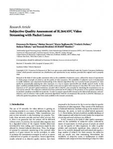
Fig. 2. Illustration of PAS shuffling: (a) parallelism based space partitioning: hyper-rectangles derived by partitioning over dimension t and t − 1; (b) normalized sliding window replication and shuffling amongst partitions; each partition is handled by a unique task of processing element P (cmp) .
Now, we define partition vector of size hp , which uniquely identifies a partition for each normalized sliding window sˆti for instance as: pti = (sgn(ˆ si,t−hp +1 ) |ˆ si,t−hp +1 | , · · · , sgn(ˆ si,t ) |ˆ si,t | ), where sgn(x) extracts the sign of its argument: sgn(x) = 1 if x ≥ 0 and sgn(x) = −1 if x < 0. Since −1 ≤ sˆi,t ≤ 1, each entry of the partition vector pti is either −1 or 1. Example 5.1: As is demonstrated in Figure 2(a) for 3D sliding windows. Suppose p(cmp) = 4 then we have hp = 2. Since hp < 3, only dimensions t and t − 1 are used to obtain 4 partitions as are shown in Figure 2(b). Each of them corresponds to one hyper-rectangle with the same colour in Figure 2(a). Thus, normalized sliding windows lying in the blue-grey hyper-rectangle are assigned to the blue partition (i.e., task P (cmp,3) ) in Figure 2(b), so on and so forth. Sliding Window Replication and Shuffling: In this part, we discuss how to judge whether a normalized sliding window should be replicated to other partitions as well as locate such relevant partitions (i.e., tasks). Let us start by defining the following terms. Let Hi ⊆ (1, . . . , hp ) be a subset of dimensions referred to as the dimension subset of a sliding window sˆti . Given a dimension subset Hi , the sub-permutation set RHi of sti is defined as
Now, each task of processing element P (pre) essentially scans each local normalized sliding window sˆti , for instance and checks the condition given by Lemma 5.1 to generate the dimension subset Hi . If Hi = ∅, sˆti is only shuffled to the task responsible for partition pti . Otherwise, Hi is used for creating the sub-permutation set RHi , and sˆti is replicated to the tasks corresponding to all the partitions present in RHi . Example 5.2: Consider Figure 2(b), sliding window sˆt3 (in blue) is contained in the partition (1, −1) and both dimension t and t − 1 of sˆt3 are not qualified for the condition in Lemma 5.1, therefore it is only shuffled to partition (1, −1). Sliding window sˆt1 (in green) is qualified on dimension t, therefore in addition to partition (−1, 1) where sˆt1 is located, it is also replicated to partition (1, 1). Likewise, sˆt2 is replicated to partitions (1, 1), (−1, 1), (−1, 1), and (−1, −1). Lastly, we provide two theorems to verify the efficiency and effectiveness of PAS approach. Theorem 5.2 (Complexity of Sliding Window Replication in PAS): Given a certain parallelism for the processing elements in SigCO, for the sliding window of each time series, PAS achieves O(1) replication independent of the sliding window size h and number of time series n. Proof Please refer [1]. Theorem 5.3 (Correctness and Completeness of PAS): Through PAS shuffling, each task of P (cmp) receives the normalized sliding windows located in the partition corresponding to this task and the sliding windows from other partitions that are significantly correlated with this task’s local ones. Therefore, the complete set of significantly correlated pairs of time series can be mined from the tasks of P (cmp) . Proof Please refer [1].
751
VI. C OMPUTING C ORRELATION M EASURES In the previous section, we know that by using PAS shuffling each task of processing element P (cmp) collects all the necessary sliding windows for finding the correlations contained in the partition corresponding to this task. In this part, we only describe the actions performed by each task of P (cmp) over its local sliding windows. A.
δ –Hypercube Structure
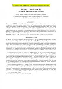
First, we introduce the δ-hypercube structure, which is exploited to prune correlation computation. We further partition the space of normalized sliding windows into δ-hypercubes, which are h-dimensional orthogonal regular hypercubes and have edges of length δ. The hypercube in which a normalized sliding window sˆti is contained, is identified by its coordinate vector, which is given as follows: �� � � �� sˆi,t−h+1 sˆi,t t ci = ,··· , . (11) δ δ All the h entries of sˆti are used in coordinate vector cti . Recall that δ is derived from significant correlation threshold �s . Given a hypercube cti , the set of its neighbouring hypercubes is denoted as N (cti ). An important property of such δ-hypercube structures is as follows: Lemma 6.1: For a normalized sliding window sˆti and its coordinate vector cti , all the sliding windows significantly correlated with sˆti are either contained in hypercube cti or the hypercubes in N (cti ). Proof Please refer [1]. Example 6.1: Figure 3(a) shows the set of the neighbouring δ-hypercubes around the red δ-hypercube, which hosts normalized sliding window sˆti (the blue star in Figure 3(a)). The red δ-hypercube associated with sˆti is located in the black partition in Figure 3(b) . B. Correlation Computation When a task of P (cmp) collects the normalized sliding windows at time instant (i.e., t), it maps these local sliding windows to different δ-hypercubes using coordinate vectors. Then, we categorize this set of hypercubes in a task as the following two types: Definition 6.1 (Home hypercube): Home hypercube is the one hosting the normalized sliding windows located in the partition corresponding to this task. Definition 6.2 (Outer hypercube): Outer hypercube is the one hosting the normalized sliding windows, which are originally located in different partitions from the partition corresponding to this task, but replicated to this task by PAS shuffling. Based on above definitions, we obtain the following observation, which is used to avoid redundant correlation computation among the tasks of processing element P (cmp) . Observation 6.1: In a task of processing element P (cmp) , the correlation computation is only needed to be performed over a pair of normalized sliding windows both from home
Fig. 3. (a) δ-hypercube (red cubic) containing normalized sliding window s ˆti (blue star) and its neighbouring δ-hypercubes (b) hypercubes containing local sliding windows in blue partition; the dotted hypercube is an outer hypercube while the others are home ones. (c) correlation computation performed in the task of P (cmp) corresponding to the blue partition.
Algorithm 1 Correlation computation in each task of P (cmp) Input: local normalized sliding windows at time instant t, δ 1: for each normalized ˆti��do � s �� sliding�window s ˆi,t−h+1 s ˆi,t t , ..., δ ; 2: derive ci = δ 3: add s ˆti to list Lcti of hypercube cti ; 4: if cti is not existent in C t then � C t is a set of hypercubes hosting sliding windows. 5: add cti to hypercube set C t ; 6: for each hypercube ctk in C t do 7: if ctk is a home hypercube then 8: perform correlation computation over pairs of sliding 9: windows in Lct ; k
10: for each k = 1, · · · , |C t | do � iterate the hypercubes in C t t 11: for each l = k + 1, · · · , |C | do 12: if ctk and ctl are both outer hypercubes then 13: continue; 14: else if ctk and ctl are qualified for Lemma 6.2 then 15: perform correlation computation over pairs of sliding 16: windows respectively from Lct and Lct ; k
l
hypercube(s) or respectively from a home and an outer hypercube, since the correlations from intra- and inter-outer hypercubes are processed by the tasks of P (cmp) hosting these outer hypercubes as home ones. Now based on above analysis we proposed the correlation computation approach (refer Algorithm 1) including two steps as follows: Intra-Hypercube Correlation: For each home hypercube in a task, the correlation computation is performed over the pairs of sliding windows from this hypercube and output the qualified time series pairs. Inter-Hypercube Correlation: for two different hypercubes (i.e, both are home hypercubes or one home and one outer hypercube), we first need a pruning criterion telling us whether there could be any significantly correlated time series pairs, out of the total pairs formed by considering the normalized sliding windows in both hypercubes together. The following lemma discusses such a criteria: Lemma 6.2 (Pruning Criterion): Given two hypercubes cti and ctj (both home hypercubes or one home and one outer hypercube), if there exists a dimension k such that |ci,k − cj,k | > 1, where k ∈ {t − h + 1, · · · , t}, then all
752
the normalized sliding windows in cti and ctj can not be significantly correlated. Otherwise, we have to compute the correlation coefficient on each pair of sliding windows in cti and ctj to verify whether they are significantly correlated. Proof Please refer [1]. Example 6.2: In Figure 3(b), we have four partitions. In the task of P (cmp) corresponding to blue partition, local sliding windows are mapped to four hypercubes, of which hypercube ct1 to ct3 are home hypercubes and ct4 is an outer hypercube, since normalized sliding windows in ct4 are replicated from the red partition. In Figure 3(c), correlation computation is first performed over individual home hypercubes. Regarding interhypercube correlation, intuitively a hypercube pair requires further examination if they share a boundary with each other. Therefore only two pairs of hypercubes, ct1 ,ct2 and ct3 ,ct4 need further examination, while other pairs can be pruned. Finally, all the qualified significantly correlated time series pairs that are emitted by tasks of processing element P (cmp) are aggregated by P (agg) as shown in Figure 1, where the duplicate pairs are removed. Such resultant time series pairs are statistically significant correlated, as is discussed in Section IV. C. Computing Alternative Correlation Measures Besides Pearson and Spearman correlation, our proposed framework is able to handle diverse correlation (or similarity) measures by adopting specific normalization processes for different measures. Limited by the space, refer [1] for details. D. Integrating Dimension Reduction Techniques Even though dimensionality reduction methods are not the focus of this paper, we briefly discuss how our framework can incorporate such techniques [12], [20]. Orthonormal transformation based dimensionality reduction (e.g., discrete Fourier transformation (DFT), random projections, etc.) can be seamlessly performed in the processing element P (pre) . Tasks of P (pre) perform dimension reduction on individual normalized sliding window and send only these dimension-reduced sliding windows to processing element P (cmp) through PAS shuffling. Then, due to the distance preserving property, processing element P (cmp) is able to perform aforementioned correlation computation over these dimension-reduced sliding windows. Therefore, our proposed framework is able to be robust to queries with variable sliding window lengths. This could be our future work. VII. C OST A NALYSIS In this part, we provide theoretical complexity analysis. Computation Cost of Processing Element P (pre) : Statistics on each time series (i.e., mean, variance) are updated in constant time. PAS only uses the first hp (hp � h) entries of each normalized sliding window to derive relevant tasks in linear time w.r.t. hp , which is independent of h and n. Communication Cost between Processing Element P (pre) and P (cmp) : The communication cost for the sliding window
of each time series is decomposed as a product of the number of replicas produced by PAS and the cost of each replica (i.e., size of a normalized sliding window). As is proved in Theorem 5.2, the number of replicas for a sliding window in PAS is independent of n and h and is bounded by the parallelism of processing element P (cmp) ( P (cmp) � n ). The cost of each replica can be optimized via dimensionreduction techniques. Overall, the communication cost in PAS is dramatically decreased compared to the naive quadratic data communication method in Section I. Note that when parallelism is increased, the amount of data that each task of P (cmp) deals with is decreased. This is because under the assumption of uniform data distribution, the number of sliding windows each task processes is approximately modelled as 2nhp , which declines as parallelism of P (cmp) (p(cmp) = 2hp ) increases. Computation Cost of Processing Element P (cmp) : Each task of P (cmp) performs correlation computation only over the sliding windows from neighbouring δ-hypercubes, thereby circumventing pair-wise computation. In Section VIII, we will experimentally show the pruning power of such method. The communication cost between processing element P (cmp) and P (agg) depends on the number of qualified time series pairs. Since this number is unknown apriori, we have to omit the analysis of P (agg) and the computation cost of hash-set based duplicate removal in P (agg) is negligible as well. VIII. E XPERIMENTAL E VALUATION In this section, we perform extensive experimental evaluation comparing SigCO with baseline approaches. Due to the space limitation, we put some of experiment results in [1]. The implementations of SigCO and baselines are done using Apache Storm. We choose Storm here, because Storm has lower processing latency compared to other distributed realtime computation system (e.g, S4, Spark Streaming, Samza) due to the one-at-a-time data processing model [3]. Moreover, Storm provides flexible interfaces which allow to develop advanced customized data processing logics. Processing and source elements are respectively implemented as bolts and spouts in Storm. A. Baselines GC: it is based on distributed group-based join [15], which optimizes the sliding window replication and enables incremental correlation computing [11]. GC computes pair-wise correlations and then performs significance tests. DFTC: This is a DFT (discrete Fourier Transform) based approach proposed in [25], but we have adapted it to the distributed setting. It has a topology consisting of three processing elements. The first element shuffles a DFT-reduced sliding window according to the grid structure. The second element computes the correlations, performs the significance test and forwards qualified pairs to the last element, where duplicate removal is performed.
753
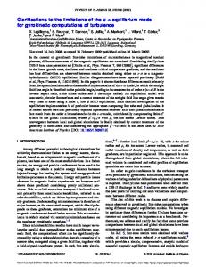
Fig. 4. Performance metrics as a function of the parameters at a constant number of input time series on real dataset. (a)-(d) communication cost and (e)-(h) processing latency.
LSHC: LSHC is based on locality sensitive hashing (LSH) [21], which use the property that the normalized sliding windows of significant correlated time series are close in Euclidean space (refer Section IV). The topology of LSHC consists of three processing elements. The first element computes the hash value of the normalized sliding windows for each hash table. Sliding windows that are mapped to a bucket in each hash table are shuffled to the same task of the second element, where the correlation computation is performed over the sliding windows in each bucket per hash table. LSHC parameters are chosen to minimize the processing latency while ensuring the failure probability (i.e., the probability of not reporting a certain qualified pair) at 5% [21]. Likewise, the last element aggregates correlated time series pairs B. Parameters and Metrics We use four evaluation parameters to establish the efficacy of SigCO: sliding window size h, query threshold �, parallelism P and the time interval Δ between time series tuples input to the engine known as the injection interval. For the fair evaluation, all the approaches have the same parallelism. For these parameters, we have a basic setup where: Δ = 2sec, h = 100, � = 0.95 and P = 8 for tuning. We use five performance metrics as follows. Communication cost is measured by the amount of data units communicated between the front two elements of each approach divided by the parallelism. Here, a data unit is a basic data type, which could be float, integer, etc. As the communication cost between the last two elements depends on the qualified time series pairs, we omit it here. Processing latency is the average processing time for each task of elements considered together. Peak capacity is the maximum number of time series that an approach can simultaneously process without causing bottlenecks in the system [3], [25]. A bottleneck is caused when sliding windows at the current time instant have
to wait (in memory) for the sliding windows at a previous time instant to finish processing [3], [25]. Bottlenecks leads the processing of the following sliding windows to lag further and further and even memory overflows. Bottlenecks caused by any tasks are detected and reported by the Storm cluster UI [3]. Replication rate is defined as the number of tuples carrying sliding windows produced by the first processing element, divided by the number of time series n. That is, the replication rate is the average number of replicas per time series sliding window communicated between the front two processing elements. Pruning power is defined as the ratio of the number of sliding window pairs that are pruned (without having to compute correlation and test significance ) to the total number of time-series pairs. Higher values of pruning power are considered better. All the performance metrics are computed by averaging every 20 seconds for 10 times, after the cluster reaches a stable state. C. Datasets and Cluster Details We use one synthetic and one real dataset for evaluations. The synthetic dataset is generated as follows. Given the n seed required number of time series n, we first generate α time series. Each seed time series is generated using a random walk model [25]. From each seed time series si , we produce α dataset as follows: sj,t = γj,t + βj · si,t , where γj,t and βj are real random numbers between [0, 100], and βj is sampled once for each time series sj , while γj,t is sampled once for each entry in time series sj . In our experiments, we set α = 1000 and n = 20000. The real dataset is the Google Cluster Usage [16] data. It records extensive activities of 12K cluster nodes from a data center over a span of 29 days. We extract three parameters:
754
CPU usage, memory usage and disk space usage for each cluster node. The total number of extracted time series is 36K. Cluster Setup: The experiments are performed using a cluster consisting of 1 master and 8 slaves. The master node has 64GB RAM, 4TB disk space and 12 x 2.30 GHz cores. Each slave node has 6 x 2.30 GHz cores, 32GB RAM and 6TB disk space. All the nodes are connected via 1GB Ethernet. D. Analysing Efficiency In this part, we present two groups of experiments. The first one compares the communication and computation cost of the approaches using constant number of input time series. Then, we vary the number of input time series to evaluate the peak capacity. Communication Cost and Processing Latency: We set constant number of time series (n = 10000) for all the experiments in this part and report the communication cost and processing latency as a function of the four parameters. For each parameter, the two metrics are measured by varying this parameter within a pre-defined range, while setting the other parameters to their basic set-up values. In Figure 4(a) and (c) the communication costs of all approaches are relatively stable w.r.t. injection interval Δ and query threshold �. The increase of parallelism enables to have more computing resource and therefore the communication cost distributed to each task is decreased. For the sliding window size h in Figure 4(d), SigCO has nearly 3x and 8x lower cost as compared to GC and DFTC at the highest level of sliding window size. Specifically, because LSHCQ requires a large number of hash tables to achieve low failure rate [21], it incurs high communication cost. As for the processing latency, in Figure 4(e), SigCO approach has nearly 2x lower latency as compared to LSHC at the maximum injection interval. Regarding the parallelism in Figure 4(f ), as its increase lowers down the average amount of data each task processes, the processing latencies of all approaches decrease. In Figure 4(g) about the query threshold �, average improvement in the latency of SigCO w.r.t. LSHC is approximately 2x. When sliding window length increases, the processing latencies of all the approaches increase as is shown in Figure 4(h). Specifically, the latency of SigCO is about 50% lower as compared to DFTC at the maximum window length. Peak Capacity: This set of experiments is to demonstrate how peak capacity of each approach varies as a function of each parameter. When a certain parameter is varied during the experiment, the other parameters are set to their basic set-up values. The peak capacity increases as a function of the injection interval and parallelism (refer Figure 5(a) and (b)). This is because their increases lead to more computing resources and available processing time interval , thereby improving peak capacity. At the highest level of parallelism and injection interval, SigCO respectively exhibits 50% and 60% more peak capacities than DFTC. In addition, the increase of query threshold has very little effect on the peak capacities of
Fig. 5. Peak capacity as a function of the parameters on real dataset.
all the approaches (refer Figure 5(c)). On the other hand, the sliding window size affects the peak capacity adversely (refer Figure 5(d)) for all approaches. This is because when the sliding window size increases, DFTC typically needs more DFT coefficients to retain the same amount of energy, and LSHC takes more time for computing hash values and correlations. And since the parallelism (or available resources) is constant in this experiment, the peak capacity drops to keep the system bottleneck free. However, in practice peak capacity can be maintained by increasing parallelism or incorporate dimension reduction techniques. E. Analysing Replication Rate As time interval and query threshold have no effects on the replication rate, this set of experiments measures the variation of replication rate w.r.t. number of input time series, parallelism and sliding window size. Figure 6(a) shows that the replication rates of all the approaches are robust to varying n. SigCO achieves around 20x less replication rate than DFTC. LSHC has 10x more replicate rate than SigCO, since it constructs large number of hash tables to attain low failure rate. In Figure 6(b), GC presents an increasing replication rate, because GC performs group-based sliding window replication, where the group scheme depends on the parallelism in order to save communication cost [15]. SigCO has a slightly increasing replication rate, which is 2x times less than GC at the maximum parallelism. In Figure 6(c), DFTC exhibits fast increasing replication rate due to its increased number of DFT coefficients and neighbouring-cell data replication [25]. The other approaches are relatively stable w.r.t. h. In summary, above results testify the theorems of PAS shuffling in Section V. One point to note is that LSHC’s replication rate is 10x larger that SigCO at most, although it is little affected by parameter variations. F. Analysing Pruning Power This set of experiments evaluates the pruning power (the higher, the better) of SigCO against DFTC and LSHC. Because
755
R EFERENCES [1] EPFL-REPORT. http://infoscience.epfl.ch/record/209946/. [2] Apache Samza. https://http://samza.apache.org/. Fig. 6. Replication rate as a function of the parameters on real dataset.
GC performs pair-wise correlation computation, we omit it here. The pruning power is directly affected by the query threshold � and sliding-window length h, thus in Table I we present the pruning power as a function of these two parameters, while Δ and P are set to their basic set-up values. The upper, middle and lower values in each cell of Table I respectively correspond to DFTC, LSHC and SigCO. In SigCO, based on the relation among �, �s and δ (refer Section IV), higher values of � lead to shrinking δ-hypercubes and therefore more pairs of sliding windows are pruned. On the other hand, higher h leads to more sparse distribution of normalized sliding windows in Euclidean space, thereby pruning more sliding window pairs [15]. Therefore, at the maximum � and h, SigCO achieves the maximum pruning power 0.817, which is around 50% better than DFTC and LSHC. TABLE I P RUNING POWERS OF DFTC, LSHC AND S IG CO AS A FUNCTION OF QUERY THRESHOLD � AND SLIDING - WINDOW LENGTH h FOR REAL DATASET.
HH h 200 � HH
400
600
800
1000
0.7: DFTC
0.421
0.436
0.423
0.454
0.427
LSHC
0.525
0.534
0.539
0.542
0.535
SigCO
0.625
0.644
0.659
0.642
0.705
0.8: DFTC
0.467
0.485
0.472
0.486
0.497
LSHC
0.535
0.544
0.551
0.548
0.535
SigCO
0.632
0.687
0.748
0.789
0.792
0.9: DFTC
0.561
0.542
0.533
0.572
0.542
LSHC
0.529
0.549
0.539
0.542
0.535
SigCO
0.676
0.718
0.748
0.788
0.817
IX. C ONCLUSION In this paper, we thoroughly investigated the problem of mining statistically significant correlations from time series using distributed real-time computation engine. Through extensive experimental evaluation against various baselines, we have established the efficiency and effectiveness of proposed SigCO approach. X. ACKNOWLEDGMENTS This work was supported by Nano-Tera.ch through the OpenSenseII project.
[3] Apache Storm. http://storm-project.net/. [4] D. Abadi, D. Carney, U. Cetintemel, M. Cherniack, C. Convey, S. Lee, M. Stonebraker, N. Tatbul, and S. Zdonik. Aurora : A new model and architecture for data stream management. VLDB Journal, pages 120– 139, 2003. [5] L. Abraham, J. Allen, O. Barykin, V. Borkar, B. Chopra, C. Gerea, D. Merl, J. Metzler, D. Reiss, S. Subramanian, et al. Scuba: diving into data at facebook. PVLDB, 6(11):1057–1067, 2013. [6] R. Cole, D. Shasha, and X. Zhao. Fast window correlations over uncooperative time series. In ACM SIGKDD, pages 743–749. ACM, 2005. [7] S. Fries, B. Boden, G. Stepien, and T. Seidl. Phidj: Parallel similarity self-join for high-dimensional vector data with mapreduce. In ICDE, pages 796–807. IEEE, 2014. [8] T. Guo, T. G. Papaioannou, and K. Aberer. Model-view sensor data management in the cloud. In Big Data, 2013 IEEE International Conference on, pages 282–290. IEEE, 2013. [9] T. Guo, S. Sathe, and K. Aberer. Fast distributed correlation discovery over streaming time-series data. In Proc. 24th ACM Int. Conf. on Information and Knowledge Management (CIKM), 2015. [10] Y.-W. Laih. Measuring rank correlation coefficients between financial time series: A garch-copula based sequence alignment algorithm. European Journal of Operational Research, 232. [11] Y. Li, M. L. Yiu, Z. Gong, et al. Discovering longest-lasting correlation in sequence databases. PVLDB Endowment, 6(14):1666–1677, 2013. [12] A. Mueen, S. Nath, and J. Liu. Fast approximate correlation for massive time-series data. In SIGMOD, pages 171–182, 2010. [13] L. Neumeyer, B. Robbins, A. Nair, and A. Kesari. S4: Distributed stream computing platform. In ICDMW, pages 170–177. IEEE, 2010. [14] T. Preis, D. Y. Kenett, H. E. Stanley, D. Helbing, and E. Ben-Jacob. Quantifying the behavior of stock correlations under market stress. Scientific reports, 2, 2012. [15] A. Rajaraman, J. D. Ullman, J. D. Ullman, and J. D. Ullman. Mining of massive datasets, volume 77. Cambridge University Press, 2012. [16] C. Reiss, J. Wilkes, and J. L. Hellerstein. Google cluster-usage traces: format+ schema. Google Inc., White Paper, 2011. [17] L. Sachs. Applied statistics: a handbook of techniques. Springer Science & Business Media, 2012. [18] Y. Sakurai, S. Papadimitriou, and C. Faloutsos. Braid: Stream mining through group lag correlations. In ACM SIGMOD, pages 599–610. ACM, 2005. [19] A. D. Sarma, Y. He, and S. Chaudhuri. Clusterjoin: A similarity joins framework using map-reduce. In PVLDB, 2014. [20] S. Sathe and K. Aberer. AFFINITY: Efficiently querying statistical measures on time- series data. In ICDE, pages 841–852, 2013. [21] N. Sundaram, A. Turmukhametova, N. Satish, T. Mostak, P. Indyk, S. Madden, and P. Dubey. Streaming similarity search over one billion tweets using parallel locality-sensitive hashing. PVLDB, 6:1930–1941, 2013. [22] Y. Wang, A. Metwally, and S. Parthasarathy. Scalable all-pairs similarity search in metric spaces. In 19th ACM SIGKDD, pages 829–837. ACM, 2013. [23] Q. Xie, S. Shang, B. Yuan, C. Pang, and X. Zhang. Local correlation detection with linearity enhancement in streaming data. In ACM CIKM, pages 309–318. ACM, 2013. [24] M. Zaharia, T. Das, H. Li, S. Shenker, and I. Stoica. Discretized streams: an efficient and fault-tolerant model for stream processing on large clusters. In 4th USENIX HotCloud, pages 10–10. USENIX, 2012. [25] Y. Zhu and D. Shasha. Statstream: Statistical monitoring of thousands of data streams in real time. In VLDB, pages 358–369, 2002.
756