grid current from an LCL-filtered Voltage Source Inverter (VSI) .... See http://www.ieee.org/publications_standards/publications/rights/index.html for more ...
This article has been accepted for publication in a future issue of this journal, but has not been fully edited. Content may change prior to final publication. Citation information: DOI 10.1109/TPEL.2017.2740946, IEEE Transactions on Power Electronics
> REPLACE THIS LINE WITH YOUR PAPER IDENTIFICATION NUMBER (DOUBLE-CLICK HERE TO EDIT)
REPLACE THIS LINE WITH YOUR PAPER IDENTIFICATION NUMBER (DOUBLE-CLICK HERE TO EDIT) < In an ICF control system, the grid current has to be regulated indirectly, which may suffer from severe distortions in case of grid-voltage harmonics, since the harmonic current can freely flow through the filter capacitor C [13], [14]. This issue can be explained by the experimental results in Fig. 1, where the inverter current i1 is controlled to zero by a Proportional Resonant (PR) controller plus resonant Harmonic Controllers (HCs). However, it is seen in Fig. 1 that the grid current i2 is significantly distorted by the grid voltage harmonics, which flows into the filter capacitor C. Due to the loss of harmonic information (i.e., the inverter current i1 contains no information of the harmonics from the grid voltage), the HCs (either resonant or repetitive controllers) are not able to mitigate the harmonics. Clearly, a straightforward way is to make the current reference contain the full harmonic information, which can be realized by calculating the capacitor current from the capacitor voltage and then adding it into the reference. This idea has been reported to be effective for the ICF control system with a novel D-Σ digital controller in [15]. To cope with the harmonic issue of the ICF control system for the LCL-filtered VSI, a feedforward scheme has been extensively explored [7], [12], [16]. A proportional grid-voltage feedforward strategy was applied in [7], which shows excellent harmonic-attenuation performance, since the LCL-filter was simply treated as an L-filter. However, its effectiveness is deteriorated when the filter capacitor is considered. As an alternative, a transfer function was derived and inserted into the feedforward loop in [16] to eliminate an undesirable admittance effect. Unfortunately, the grid current may still be distorted by grid voltage harmonics, since the feedforward term is the capacitor voltage rather than the grid voltage. In [12], an accurate feedforward function for the grid voltage was derived, which can fully mitigate the impacts of grid voltage distortions on the grid current. However, a second-order differentiator is required in order to synthesize the feedforward function in [12]. Such a second-order differentiator is sensitive to noises, making the method impractical. Although an alternative capacitor-current feedforward scheme was also presented in [12] to tackle this issue, it is still impractical considering the increased cost because of the necessary capacitor-current measurement. In light of the above discussions, this paper proposes an enhanced scheme for the grid-current harmonic mitigation of the ICF controlled VSIs. Compared with the feedforward scheme in [12], only one differentiator is needed in the proposed scheme. Since the differentiator mainly works on the low-order harmonics, its noise sensitivity can be significantly reduced with an adjustable differentiator [17]. Furthermore, a harmonic compensation loop is added in the proposed scheme in order to provide the harmonic information needed for the resonant harmonic controllers. In spite of this added loop, the stability characteristic of the proposed control system can remain as that of the original system owing to a special design of the compensation position. Actually, the proposed control system is equivalent to a system applying the proportional control to the inverter current while the resonant control to the grid current. Therefore, the parameter design of the proposed
2
control system can be simplified to that of the typical single-loop ICF control system. The rest of this paper is organized as follows: Section II presents the modelling of the typical single-loop ICF control system for the LCL-filtered VSI, with which the grid harmonic impedance of the system is derived and its insufficient harmonic attenuation capability is analyzed in details. The stability characteristic of the system is also briefly discussed. In Section III, a simple capacitor-current compensation scheme is explored for harmonic attenuation of the ICF control system, which however may cause instability. To solve this issue, an improved control scheme is then developed. The parameter design of the LCL-filter and the controllers is presented in Section IV before the experimental verification in Section V and conclusion in Section VI.
(a)
(b) Fig. 2. Three-phase LCL-filtered grid-connected inverter: (a) general structure of the system with either inverter or grid current feedback control, and (b) equivalent block diagram of the Inverter Current Feedback (ICF) control.
II. SYSTEM MODELLING AND PROBLEM ANALYSIS Fig. 2(a) shows the general structure of a three-phase VSI system, which is connected to the grid through an LCL-filter. Its typical applications can be found in the DC/AC stage of transformerless string PV inverters [18]. Those inverters are required to comply with relevant grid standards, such as the IEEE-1547 Standard, which specifies the limits of both lowand high-frequency harmonics in the output current of the inverter [18]. As also observed in Fig. 2(a), the inverter current, which should be sensed for overcurrent protection, is used cost-effectively for control in most commercial products. In this case, the current controller is implemented in the αβ frame, which consists of a proportional controller and a set of resonant controllers for harmonic compensation. The resonant controllers produce infinite gains at the specified frequencies. Therefore, when the harmonic contents of the reference signal are set to zero, the inverter current i1 should be free of low-order
0885-8993 (c) 2017 IEEE. Personal use is permitted, but republication/redistribution requires IEEE permission. See http://www.ieee.org/publications_standards/publications/rights/index.html for more information.
This article has been accepted for publication in a future issue of this journal, but has not been fully edited. Content may change prior to final publication. Citation information: DOI 10.1109/TPEL.2017.2740946, IEEE Transactions on Power Electronics
> REPLACE THIS LINE WITH YOUR PAPER IDENTIFICATION NUMBER (DOUBLE-CLICK HERE TO EDIT) < harmonic distortion in steady state. On the other hand, the grid current i2 has to be regulated indirectly with additional errors, which may be distorted in the presence of grid voltage harmonics. The entire current controller F(s) (i.e., the PR controller plus HCs) is given as J
F s K p h 1
K rh s
s 2 h0
A. Modelling of the Control System With the symbols defined in Fig. 2, the inverter system can be described by the following transfer functions in s-domain as (2) v F s e sT i i1 d
sL1i1 v vC
(3)
sL2i2 vC vg
(4)
sCvC i1 i2 (5) where the grid impedance is included in the grid-side inductor L2 and the filter parasitic resistances are neglected (considered as the worst case). The grid voltage can be taken as a disturbance. Besides, Td is the total time delay of the system, which can be approximated as 1.5Ts by considering the process of sampling, computation, updating of the compare registers, and zero-order-hold effect of the Pulse-Width Modulation (PWM) [19]. The scalar notation of all variables is used for convenience, which should be interpreted as space vectors for the αβ-frame implementation. With the above transfer functions, the control block diagram of the ICF control system is shown in Fig. 2(b). The inverter current and the grid current can be calculated from the reference current and grid voltage, which are then given as F (s)e sTd G1 (s) G1 (s)G2 (s) i1 i vg (6) sTd 1 F (s)e G1 (s) 1 F (s)e sTd G1 (s) F ( s )e
sTd
G1 ( s)G2 ( s)
1 F ( s )e
with G1 ( s)
sTd
G1 ( s)
i
G1 ( s)G22 ( s)
1 F ( s )e
sTd
G1 ( s)
which is contrary to the characteristics of the single-loop GCF control system as shown in Fig. 3(b).
(1)
2
where Kp, h, Krh, J and ω0 represent the proportional gain, harmonic order, resonant gain of each harmonic component, maximum harmonic order specified for attenuation, and the fundamental grid frequency, correspondingly.
i2
3
sCG2 ( s ) vg
(a) (b) Fig. 3. Stable and unstable regions of the system with (a) ICF and (b) GCF.
To illustrate it more clearly, the root loci of the single-loop ICF control system are plotted in Fig. 4 for six resonance frequencies obtained with different filter capacitances shown in Table I. According to Fig. 3, it can be observed from Fig. 4(a) and (b) that the first three cases in Table I can be stable with a properly designed Kp, since the resonance frequencies are all below the critical frequency (fc = fs/6 = 3.33 kHz). On the other hand, as seen from Fig. 4(c) and (d), the other three cases are always unstable regardless of the value of Kp, since their resonance frequencies are all above the critical frequency. Detailed theoretical analysis of the stability characteristics of the single-loop ICF and GCF control systems has been given in [19], [22], which will be not elaborated in this paper. TABLE I LCL PARAMETERS AND RESONANCE FREQUENCIES OF SIX CASES Case Case Case Case Case Case I II III IV V VI Inverter-side inductor 1.1 1.1 1.1 1.1 1.1 1.1 L1 (mH) Grid-side inductor 1.1 1.1 1.1 1.1 1.1 1.1 L2 (mH) Capacitor 20 12 8 4 3 2 C (µF) Resonance frequency 1.52 1.96 2.40 3.39 3.92 4.80 fr (kHz)
(7)
1 s 2 L2 C 1 and G2 ( s ) 2 . 3 s L2 C 1 s L1 L2 C s L1 L2 (a)
B. Stability Characteristic of the ICF Control System Stabilities of the single-loop current control systems of the LCL-filtered VSI have been widely studied [19]–[22]. Specifically, for the single-loop ICF control, the system can be stable with a properly designed proportional controller gain as long as the LCL-filter resonance frequency is smaller than the critical frequency fc. The critical frequency fc is the frequency at which the phase of the open-loop transfer function reaches 180, and it is mainly determined by the value of the time delay in a digital system [19], [20]. For instance, for an ICF control system with a time delay of 1.5Ts, fc can be calculated to be fs/6. In this case, the stable region of the system is (0, fs/6) and the unstable region is (fs/6, fs/2) as shown in Fig. 3(a),
(b)
(c) (d) Fig. 4. Root loci of the ICF control system when the LCL-filter resonance frequency is (a) below the critical frequency, and (c) above the critical frequency, where (b) and (d) are the zoomed-in root loci of (a) and (c), respectively.
0885-8993 (c) 2017 IEEE. Personal use is permitted, but republication/redistribution requires IEEE permission. See http://www.ieee.org/publications_standards/publications/rights/index.html for more information.
This article has been accepted for publication in a future issue of this journal, but has not been fully edited. Content may change prior to final publication. Citation information: DOI 10.1109/TPEL.2017.2740946, IEEE Transactions on Power Electronics
> REPLACE THIS LINE WITH YOUR PAPER IDENTIFICATION NUMBER (DOUBLE-CLICK HERE TO EDIT) < C. Harmonic Impedance Analysis For ICF control, the inverter current can be free of low-order distortion with the benefit of HCs, no matter what harmonic sources are from the inverter-side or the grid-side. Specially, in case of inverter-side disturbance (e.g. dead-time effect), the grid current can also be free of distortion as long as the low-order harmonics have been eliminated from the inverter current before they flow into the grid-side inductor. However, in case of the grid-voltage distortion, the grid-current harmonics cannot be rejected by the HCs any more, due to the uncontrolled harmonic currents in the filter capacitor. To further elaborate the grid-current harmonic attenuation ability of the ICF control system, the grid harmonic impedance is calculated from (7) and it can be given as Zg
vg i2
s 3 L1 L2 C s L1 L2 F (s )e s 2 L1C sCF ( s )e
sTd
sTd
s L C 1 2
2
1
(8)
which indicates the relationship between the grid voltage and the resulting grid current [12]. According to (8), at low and high frequencies, the harmonic impedance can be approximated as (9) and (10), respectively, vg Z gLow K p (9) i2
Z gHigh
4
Fig. 5. Equivalent circuit of the grid-connected LCL-filtered voltage-source inverter with its inverter current controlled by the proportional-resonant controller plus resonant Harmonic Controllers (HCs).
Furthermore, Fig. 6 shows the Bode plot of the grid impedance Zg, which compares the harmonic impedances of the ICF control systems whose harmonic controllers are disabled and enabled, respectively. The controllers are designed according to [24], which results in 10.69 for Kp. The fundamental resonant controllers of the two systems are disabled in order to clearly distinguish the difference induced by the harmonic controllers.
vg
sL2 (10) i2 It can be seen from (9) and (10) that the harmonic impedance shows resistive characteristic at low frequencies and inductive characteristic at high frequencies. The resistance is determined by Kp, while the inductance is determined by the grid-side inductor L2. For a specific case, at the frequencies where the HCs work, F(s) becomes infinite and (8) can be approximated as vg 1 Z gHarmonic sL2 (11) i2 sC These three characteristics can be intuitively illustrated using the circuit model of the control system presented in [23], where the principle of the PR controller is represented by a resistor and a set of LC circuits in Fig. 5. The findings from this equivalent circuit can be concluded as follows: 1) At very low frequencies, the inductor impedance is very small and the capacitor impedance is very large, which is seen as a short circuit and an open circuit system, respectively. In this case, the current contributed by the grid voltage mainly flows in loop A, whose impedance is dominated by the resistor with the value of Kp (see (9)). 2) At very high frequency, the capacitor is seen as a short circuit, and thus the current contributed by the grid voltage mainly flows in loop B, whose impedance is dominated by L2 (see (10)). 3) At frequencies where the HCs work, the impedance of the LC circuits become infinite. Thus, the current contributed by the grid voltage mainly flows in loop B whose impedance is dominated by L2 and the filter capacitor C (see (11)).
Fig. 6. Bode diagram of the grid harmonic impedance for the ICF control system when the HCs are enabled and disabled.
It can be observed from the Bode plot that the characteristic of the grid impedance is in agreement with the theoretical analysis, which behaves as a resistor at low frequencies and an inductor at high frequencies. It is noted that at the working frequencies of the HCs, the harmonic impedance of the system is slightly larger than that when the HCs are disabled, because the current contributed by the grid voltage can flow both in loop A and loop B when the HCs are disabled, which has a lower impedance than loop B due to the parallel topology. It can be concluded that, although the HCs of the ICF control system cannot reject the grid-current harmonics completely, they help to attenuate the harmonics to some extent. However, the attenuation is quite limited, which is always below 40 dB in the provided case. Moreover, at the working frequencies of HCs, the impedance values are only determined by L2 and C (see (11) and Fig. 5), since the grid-current harmonics only flows from L2 to C when the HCs are enabled. Therefore, the harmonic attenuation capability is fixed by the filter parameters and cannot be improved by designing the controller parameters. Unfortunately, in commercial products, to obtain a similar filtering performance, a comparatively large capacitor is preferred instead of a large grid-side inductor in order to reduce
0885-8993 (c) 2017 IEEE. Personal use is permitted, but republication/redistribution requires IEEE permission. See http://www.ieee.org/publications_standards/publications/rights/index.html for more information.
This article has been accepted for publication in a future issue of this journal, but has not been fully edited. Content may change prior to final publication. Citation information: DOI 10.1109/TPEL.2017.2740946, IEEE Transactions on Power Electronics
> REPLACE THIS LINE WITH YOUR PAPER IDENTIFICATION NUMBER (DOUBLE-CLICK HERE TO EDIT) < the volume and cost of the filter. As a result, the harmonic impedance will be small according to (11). Simulations are carried out to further illustrate this, and the results are given in Fig. 7, where the ICF control is employed for the LCL-filter in Table I with the resonance frequency of 1.52 kHz and the grid voltage is distorted by the typical 5th, 7th, and 11th harmonics whose magnitudes are all 5% of the fundamental component. Due to the severe grid voltage distortion, both the inverter current and the grid current are seriously distorted without the HCs. The HCs are then enabled at 0.02 s, and the low-order harmonics in the inverter current can effectively be rejected, owning to the infinite gains introduced by HCs. However, the grid current is still distorted in that case, due to the limited harmonic impedance (decided by L2 and C according to (11)) at the harmonic frequencies.
5
control system, since the measured inverter current i1 and the estimated capacitor current ic form the grid current i2. As a result, the infinite harmonic impedance for the ICF control system can be introduced at the frequencies where the HCs work and the harmonic components can therefore be rejected. Fig. 9 shows the Bode plot of the grid harmonic impedance, which compares the impedances of the system with and without the compensation loop. As evidenced in Fig. 9, the infinite harmonic impedance can only be introduced when the compensation loop is added.
Fig. 8. Three-phase ICF-controlled LCL-filtered grid-connected inverter with capacitor-current compensation.
Fig. 7. Simulation waveforms of the inverter current and the grid current when the HCs are enabled after 0.02 s in the ICF control system.
III. PROPOSED GRID-CURRENT HARMONIC SUPPRESSION METHOD FOR ICF CONTROL SYSTEM This section introduces a simple capacitor-current compensation term to the ICF control system, which enables the system to generate infinite harmonic impedance at the working frequencies of HCs. However, despite its simplicity, the control system may become unstable. Accordingly, an improved control scheme is developed to address this issue, which inherits the stability characteristic of the typical ICF control system while the grid-current harmonic attenuation capability is enhanced. A. Capacitor-Current Compensation Generally, for unity power factor operation, the inverter current reference of the ICF control system should be changed to include the fundamental reactive capacitor current which is usually calculated from the fundamental grid voltage. Similarly, this idea can be used in the ICF control system for grid-current harmonic control, for which the inverter reference should be changed to include the full capacitor current. To implement it, no extra sensor is added, since the capacitor current can be calculated from the capacitor voltage, which has been measured for grid synchronization. The resultant control diagram is shown in Fig. 8, which is equivalent to the single-loop GCF
Fig. 9. Bode diagram of the grid harmonic impedance for the ICF control system when capacitor-current compensation is enabled and disabled.
However, the above approach is not commonly adopted in typical PR or PI controlled ICF systems in literature, which may be because of the instability risk introduced by the compensation loop. Specifically, since the modified system is equivalent to the GCF system, its stable region is also the same as the GCF, which is (fs/6, fs/2) rather than (0, fs/6). In this case, additional damping is required to ensure the system stability under weak grid conditions. This is explained in the following. The root loci of the modified system are plotted in Fig. 10 with the first three LCL-filters in Table I, whose resonance frequencies are in the stable region of the single-loop ICF control system. However, it is observed in Fig. 10 that the system with the compensation loop cannot be stable with these three LCL-filters regardless of the value of Kp. The instability is further verified by the simulation results in Fig. 11, where the HCs are always enabled during the simulation and the grid
0885-8993 (c) 2017 IEEE. Personal use is permitted, but republication/redistribution requires IEEE permission. See http://www.ieee.org/publications_standards/publications/rights/index.html for more information.
This article has been accepted for publication in a future issue of this journal, but has not been fully edited. Content may change prior to final publication. Citation information: DOI 10.1109/TPEL.2017.2740946, IEEE Transactions on Power Electronics
> REPLACE THIS LINE WITH YOUR PAPER IDENTIFICATION NUMBER (DOUBLE-CLICK HERE TO EDIT) < condition is the same as that in Fig. 7. The compensation loop is enabled at 0.02 s and the instability occurs immediately, since (0, fs/6) has become the unstable region of the modified system. In practice, the resonance frequency may reduce below the critical frequency due to the increase of the grid impedance under weak grid conditions, which may trigger the instability of the modified control system.
6
Fig. 13 with the first three LCL-filter parameters in Table I. It can be seen that the system can be stable with a proper Kp in the proposed method. Besides, the root loci are almost the same with that of the single-loop ICF control system as shown in Fig. 4(a) and (b), i.e., stable region of the proposed system is in agreement with the typical single-loop ICF control system despite an additional compensation loop.
(a) (b) Fig. 10. Root loci of the ICF control system with the capacitor-current compensation when the LCL-filter resonance frequency is below the critical frequency, (a) full root loci (b) zoomed-in root loci. Fig. 12. Three-phase ICF-controlled LCL-filtered grid-connected inverter with the proposed capacitor-current compensation.
(a) Fig. 11. Simulation waveforms of the inverter current and the grid current when the capacitor-current compensation is enabled after 0.02 s in the ICF control system.
B. Proposed Scheme To avoid the instability issue of the modified system, an intuitive solution is to insert multiple band-pass filters into the iC compensation loop, which only allow the predefined harmonics to pass. However, as the number of the harmonics to be attenuated increases, the computational burden and the design difficulty become significant. To avoid these issues, a simpler scheme is proposed in the following, which has the same computational effort with the method illustrated in Fig. 8 but a different compensation position as shown in Fig. 12. In the proposed method, the capacitor current is only processed by the resonant controllers instead of the proportional controller. The resonant HCs work on low-order harmonics, whose resonant frequencies are below the system bandwidth in order to ensure the controllability. When the resonant controllers are properly designed, their associated phase lags are nearly negligible and the stability of the control system will be mainly determined by the proportional gain Kp [11], [22]. In this case, the added compensation loop will not affect the stable and unstable regions of the initial single-loop ICF control system due to the same proportional gain. This can be observed from the root loci of the proposed control system in
(b)
Fig. 13. Root loci of the ICF control system with the proposed capacitorcurrent compensation when the LCL-filter resonance frequency is below the critical frequency, (a) full root loci (b) zoomed-in root loci.
However, in terms of harmonic attenuation, the proposed scheme is superior to the single-loop ICF control system, as observed from the Bode plots in Fig. 14, where the infinite impedance is obtained at the working frequencies of the HCs due to the grid harmonic information indirectly provided by the compensation loop. Looking back at Fig. 12, it is interesting to find that the proposed scheme is actually a combination of an ICF control system and a GCF control system (the inverter current is controlled by the proportional controller, while the grid current is controlled by the resonant controllers). That is to say, the proposed scheme inherits the stability characteristic of the single-loop ICF control system and the harmonic attenuation capability of the single-loop GCF control system. To validate the theoretical analysis, simulation results are given in Fig. 15. It can be seen that, without the proposed method, the HCs can only reject the low-order harmonics in the inverter current, and fail to reject the grid current distortions. For comparison, the proposed scheme is then enabled at 0.02 s. Clearly, the system maintains the stability and the grid current becomes sinusoidal. In principle, similar results can also be obtained by the accurate grid-voltage feedforward scheme in [12], but a second-order differentiator is required, which may
0885-8993 (c) 2017 IEEE. Personal use is permitted, but republication/redistribution requires IEEE permission. See http://www.ieee.org/publications_standards/publications/rights/index.html for more information.
This article has been accepted for publication in a future issue of this journal, but has not been fully edited. Content may change prior to final publication. Citation information: DOI 10.1109/TPEL.2017.2740946, IEEE Transactions on Power Electronics
> REPLACE THIS LINE WITH YOUR PAPER IDENTIFICATION NUMBER (DOUBLE-CLICK HERE TO EDIT) < cause noise amplification and usually it is difficult to implement. Although a capacitor current based approach was also proposed in [12] to avoid derivatives, that method is different from the proposed one. The capacitor current in [12] was used for an approximate implementation of the grid-voltage feedforward control, while in the proposed control system, the capacitor current is used for harmonic reference generation and HCs should be used at the same time. Compared with the proposed method, the method in [12] suffers from inaccuracy, design complexity and additional cost for current sensing.
7
method to the phase error is unknown, which should be investigated to ensure an accurate harmonic control. Detailed investigation will be provided in Section V. D. Performance Evaluation of the Proposed Scheme Simulations are carried out to further evaluate the performance of the proposed method, and the results are shown in Fig. 16. It is seen from Fig. 16(a) and (b) that the THD of the grid current without the proposed scheme is 6.6 % in the first case (grid-voltage THD = 3.46 %, deadtime 0.5 us), which in contrast reduces to 1.99 % with the proposed scheme. Furthermore, when the grid voltage THD increases to 6.4 %, the grid current THD increases simultaneously to 12.65 % without the proposed scheme, while it is only 2.01 % with the proposed scheme, as seen from Fig. 16(c) and (d). Moreover, it is observed from Fig. 16(e) and (f) that, when the grid voltage is highly distorted with a THD of 12.25 %, the THD of the grid current rises to 28.27 %. By contrast, when the proposed method is adopted, it is reduced to only 2.73 %. In all, the effectiveness of the proposed method is verified by the simulations. IV. PARAMETER DESIGN OF THE LCL-FILTER AND CURRENT CONTROLLER
Fig. 14. Bode diagram of the grid harmonic impedance for the ICF controlled system when the proposed method is enabled and disabled.
A. LCL-Filter Design In practice, the switching ripple current should be limited within 15 % ~ 40 % of the rated current [11], [25]–[27]. To realize it, the relationship between the ripple current and L1 has been derived in [28], where the peak ripple current value is given as i1a
Fig. 15. Simulation waveforms of the inverter current and the grid current when the proposed method is enabled after 0.02 s in the ICF control system.
C. Digital Differentiator To calculate the capacitor current, a differentiator is needed in the proposed method. Traditional discretization methods of the differentiator suffer from either large phase error or noise amplification. To tackle this problem, an adjustable digital differentiator based on the non-ideal Generalized Integrator (GI) was developed in [17], which is used in the proposed control system for capacitor current calculation. The proposed control system is not so sensitive to the magnitude error introduced by the digital differentiator, since the magnitude error can be eliminated by the integration characteristic of the resonant controllers. On the other hand, the sensitivity of the proposed
3MvdcTsw 12 L1
(12)
in which M is the modulation ratio, vdc is the dc-bus voltage, and Tsw is the switching period. In this paper, the ripple current is designed to be 35 % of the rated current. With the parameters in Table II, the required inductance can be calculated to be 1.1 mH. Furthermore, the capacitor current is restricted to be 5 % ~ 15 % of the rated current [26], [27]. In this paper, this restriction is set to be 12 %, resulting in a capacitance of 20 µF. Finally, the grid-side inductor is designed to guarantee that the dominated switching harmonics can be well attenuated below the value required by the grid standard [28]. Considering that the high-order harmonics (above 35th order) should be limited within 0.3 % according to the grid standard, e.g., the IEEE 1547, a conservative design of 0.1 % is selected, and the minimum required grid-side inductance L2 can be calculated as 241 uH. It is noted that the required grid-side inductance is very small owing to the excellent high-frequency attenuation performance of the LCL-filter. However, a small grid-side inductor will lead to a small grid harmonic impedance and the system will be sensitive to grid voltage harmonics. Moreover, a very small grid-side inductance also makes the system quite sensitive to the grid impedance variation. Considering these issues, the grid-side inductor is designed to be identical to L1 in the experimental setup, which is also suggested by the authors of [11].
0885-8993 (c) 2017 IEEE. Personal use is permitted, but republication/redistribution requires IEEE permission. See http://www.ieee.org/publications_standards/publications/rights/index.html for more information.
This article has been accepted for publication in a future issue of this journal, but has not been fully edited. Content may change prior to final publication. Citation information: DOI 10.1109/TPEL.2017.2740946, IEEE Transactions on Power Electronics
> REPLACE THIS LINE WITH YOUR PAPER IDENTIFICATION NUMBER (DOUBLE-CLICK HERE TO EDIT)
REPLACE THIS LINE WITH YOUR PAPER IDENTIFICATION NUMBER (DOUBLE-CLICK HERE TO EDIT)
REPLACE THIS LINE WITH YOUR PAPER IDENTIFICATION NUMBER (DOUBLE-CLICK HERE TO EDIT) < Fig. 19(a) shows the inverter current and the grid current under an ideal grid condition. Because of the resonant HCs for the dead-time effect mitigation, the THD of the injected grid current is only 0.6 % under the ideal grid condition, which is much lower than the 5 % required by the grid standard. In comparison, the grid voltage output from the simulator is then set to be distorted by the low-order harmonics (5th, 7th, and 11th, THD ≈ 4.9 %) in Fig. 19(b). It is noted that both the grid current and the inverter current become seriously distorted without the HCs. Specifically, a THD of 9.9 % is observed in the grid current in Fig. 19(b), which exceeds 5 % required by the grid standard, showing the severe influence of the grid-voltage harmonics on the grid current quality. To mitigate these harmonics, the conventional resonant HCs tuned at the 5th, 7th, and 11th harmonic frequencies are enabled in Fig. 19(c). As a result, the inverter-current becomes less distorted due to the infinite harmonic impedance provided by the HCs. However, the HCs fail to mitigate the grid-current distortion, which becomes even more serious with the THD increased to 12.3 % as shown in Fig. 19(c), as previously discussed in this paper. The proposed scheme is then enabled in Fig. 19(d), where the capacitor current is calculated from the GI-based differentiator and fed forward to the input of the resonant controllers. Since the capacitor current contains the harmonic information, the proposed scheme ensures that all harmonics are produced from the inverter side rather than the grid side. As a result, the grid current can be free of distortions in theory. Clearly, it is observed from Fig. 19(d) that, with the proposed method, the grid current becomes much close to sinusoidal, which has a THD of 2.8 %. The experimental results are in agreement with the theoretical analysis and the simulation results in Section III. Hence, the effectiveness of the proposed method in case of grid voltage distortions is validated. Next, for comparison, the capacitor current is fed forward to the current reference rather than the input point of the resonant controllers. Although this approach is reported to be effective for an ICF control system using a D-Σ controller, it makes the traditional PR-controlled CCF system unstable according to the previous theoretical analysis. This conclusion is now validated
10
by the experimental results in Fig. 20, where it is observed that the system cannot be stable when the capacitor-current compensation is enabled, and finally the divergent oscillation of the inverter current triggers the overcurrent protection. Again, the experimental results are in agreement with the simulation result in Fig. 11, which also validates the theoretical analysis.
Fig. 20. Experimental waveforms of the inverter current and the grid current when the capacitor-current compensation is enabled.
To give a more comprehensive comparison, for the three control schemes used in Fig. 19, the THD of the grid current are measured at different operating points: from 10 % to 100 % of the rated power. The grid voltage distortion is the same with that in the previous experiments. The results are presented in Fig. 21, where it can be observed that the proposed method has the lowest THD at all operating points among the three control schemes. Specifically, above 30 % of the rated power, the proposed method can guarantee the THD to be lower than 3 %, while for the other two control systems, the THD are almost higher than 10 %. Although the relative THD of the proposed method at 10 % of the rated power is 12.21 %, its corresponding absolute value becomes 1.2%, which is still lower than required in the grid standard. Besides, it is noted that, above 60 % of the rated power, the use of HCs even worsens the grid current quality as a higher THD is observed compared with the system without HCs. Additionally, the phase errors introduced by the non-ideal GI
Fig. 21. THD of the grid current i2 for three different control systems at different operating point.
0885-8993 (c) 2017 IEEE. Personal use is permitted, but republication/redistribution requires IEEE permission. See http://www.ieee.org/publications_standards/publications/rights/index.html for more information.
This article has been accepted for publication in a future issue of this journal, but has not been fully edited. Content may change prior to final publication. Citation information: DOI 10.1109/TPEL.2017.2740946, IEEE Transactions on Power Electronics
> REPLACE THIS LINE WITH YOUR PAPER IDENTIFICATION NUMBER (DOUBLE-CLICK HERE TO EDIT) < digital differentiator with four different k values are compared in Fig. 22. Transfer function of the non-ideal GI differentiator is given by [17] 2 s (14) GI s 2 s ks 2 where ωʹ is the Nyquist frequency and k is used to tune the phase and magnitude response of the differentiator. For digital implementation, the first-order hold discretization method is used to discretize (14). It can be seen from Fig. 22 that a larger k value leads to a larger phase error. With the same k value, the phase error increases with the increase of the frequency.
11
30000 in the previous experiments considering the trade-off between the noise amplification and control performance.
(a)
Fig. 22. Phase error of the GI-based differentiator with different k values at the characteristic low-order harmonics.
(b) Fig. 24. Experimental waveforms to show the switching ripple in the inverter current and the capacitor current, (a) full view and (b) the zoom-in view of the middle zero-crossing point in Fig. 24(a).
Fig. 23. THD of the grid current at different operating point and with the differentiator tuned by four different k values.
To investigate the influence of the phase error on the control performance, the differentiator with four k values are tested in the experiments using the proposed control system. The grid condition is the same with previous experiments. With different k, the THDs of the grid current at different operating points are recorded in Fig. 23. It is seen from Fig. 22 that the phase error at the 11th harmonic is larger than 3 % for k = 50000 and 0.3 % for k = 5000. Despite the large difference, it is interesting to see in Fig. 23 that the THDs of the grid current at different operating points are quite similar. In Fig. 23, the phase error at the 19th harmonic when k is 30000 can still be maintained around 3 %, which is similar to the phase error at the 11th harmonic when k is 50000. Therefore, k is finally set to be
The designed LCL-filter is further verified experimentally. With the parameters in Table II, the rated inverter current is calculated to be 11.36 A. According to the analysis in Section IV, the ripple current can be limited to 35 % (3.98 A) of the rated current with an inverter-side inductor of 1.1 mH. To verify this, the inverter current and the capacitor current are shown in Fig. 24(a), where the switching ripple is observed clearly. Since most of the ripple currents flow into the capacitor, the maximum ripple can be observed to be 4 A from the capacitor-current waveform. The zoomed-in view of the inverter current at the middle zero-crossing point is shown in Fig. 24(b), where the ripple amplitude is 3.6 A. These results are in close agreement with the theoretical analysis. Fig. 25(a) further shows the dynamic performance of the proposed control system, where a step change in the inverter reference is enabled. The output power is changed from half load to full load. Fig. 25(b) shows the zoomed-in view of Fig. 25(a). It can be seen from these results that the injected current can quickly track the reference within 2 ms with a very small overshoot, showing also the excellent dynamic response of the proposed method.
0885-8993 (c) 2017 IEEE. Personal use is permitted, but republication/redistribution requires IEEE permission. See http://www.ieee.org/publications_standards/publications/rights/index.html for more information.
This article has been accepted for publication in a future issue of this journal, but has not been fully edited. Content may change prior to final publication. Citation information: DOI 10.1109/TPEL.2017.2740946, IEEE Transactions on Power Electronics
> REPLACE THIS LINE WITH YOUR PAPER IDENTIFICATION NUMBER (DOUBLE-CLICK HERE TO EDIT)
REPLACE THIS LINE WITH YOUR PAPER IDENTIFICATION NUMBER (DOUBLE-CLICK HERE TO EDIT) < [23] Z. Zeng, B. Hu, H. Li, L. Ran, W. Shao, and W. Zhao, “Analysis on controller of grid-connected inverter by using virtual circuit,” in Proc. EPE’15- ECCE Europe, 2015, pp. 1-8. [24] D. G. Holmes, T. A. Lipo, B. P. McGrath, and W. Y. Kong, “Optimized design of stationary frame three-phase ac current regulators,” IEEE Trans. Power Electron., vol. 24, no. 11, pp. 2417–2426, Nov. 2009. [25] A. A. Rockhill, M. Liserre, R. Teodorescu, and P. Rodriguez, “Grid-filter design for a multi-megawatt medium-voltage voltage-source inverter,” IEEE Trans. Ind. Electron., vol. 58, no. 4, pp. 1205–1217, Apr. 2011. [26] T. Wang, Z. Ye, G. Sinha, and X. Yuan, “Output filter design for a grid-interconnected three-phase inverter,” in Proc. IEEE PESC, 2003, vol. 2, pp. 779–784. [27] A. K. Sahoo, A. Shahani, K. Basu, and N. Mohan, “LCL filter design for grid-connected inverters by analytical estimation of PWM ripple voltage,” in Proc. IEEE APEC, 2014, pp. 1281–1286. [28] X. Ruan, X. Wang, D. Pan, D. Yang, W. Li, and C. Bao, Control Techniques for LCL-Type Grid-Connected Inverters, 1st ed. Beijing, China: Science Press, 2015.
Zhen Xin (S’15–M’17) was born in Shandong Province, China. He received the B.S. and M.S. degrees in electrical engineering from China University of Petroleum, China, in 2011 and 2014, respectively, and the Ph.D. degree in electrical engineering from Aalborg University, Denmark, in 2017. In 2016, he was a Visiting Scholar at University of Padova, Italy. Since June 2017, he has been with the Chinese University of Hong Kong, Hong Kong, as a Postdoctoral Research Fellow. His research interests include power quality, modeling and control of power converters for renewable energy systems, gate-driver design for SiC MOS devices, and Rogowski current sensor.
Paolo Mattavelli (S’95–A’96–M’00–SM’10–F’15) received the Ph.D. degree in electrical engineering from the University of Padova (Italy) 1995. From 1995 to 2001, he was a researcher at the University of Padova. From 2001 to 2005 he was an associate professor the University of Udine, where he led the Power Electronics Laboratory. In 2005 he joined the University of Padova in Vicenza with the same duties. From 2010 to 2012 he was a professor and member of the Center for Power Electronics Systems (CPES) at Virginia Tech. He is currently (2015) a professor at the University of Padova, leading the Power Electronics Lab. in Vicenza. His major field of interest includes analysis, modeling and analog and digital control of power converters, grid-connected converters for renewable energy systems and micro-grids, high-temperature and high-power density power electronics. In these research fields, he has been leading several industrial and government projects. From 2003 to 2012 he served as an Associate Editor for IEEE Transactions on Power Electronics. From 2005 to 2010 he was the IPCC (Industrial Power Converter Committee) Technical Review Chair for the IEEE Transactions on Industry Applications. For terms 2003-2006, 2006-2009 and 2013-2015 he has been a member-at-large of the IEEE Power Electronics Society’s Administrative Committee. He also received in 2005, 2006, 2011 and 2012 the Prize Paper Award in the IEEE Transactions on Power Electronics and in 2007, the 2nd Prize Paper Award at the IEEE Industry Application Annual Meeting. He is an IEEE Fellow
13
Yongheng Yang (S’12–M’15) received the B.Eng. degree in electrical engineering and automation from Northwestern Polytechnical University, China, in 2009 and the Ph.D. degree in electrical engineering from Aalborg University, Denmark, in 2014. He was a postgraduate with Southeast University, China, from 2009 to 2011. In 2013, he was a Visiting Scholar at Texas A&M University, USA. Since 2014, he has been with the Department of Energy Technology, Aalborg University, where currently he is an Assistant Professor. His research includes grid integration of renewable energy systems, power electronic converter design, analysis and control, and reliability in power electronics. Dr. Yang is a Member of the IEEE Power Electronics Society (PELS) Young Professionals Committee. He served as a Guest Associate Editor of IEEE JOURNAL OF EMERGING AND SELECTED TOPICS IN POWER ELECTRONICS and a Guest Editor of Applied Sciences. He is an Associate Editor of CPSS TRANSACTIONS ON POWER ELECTRONICS AND APPLICATIONS.
Frede Blaabjerg (S’86–M’88–SM’97–F’03) was with ABB-Scandia, Randers, Denmark, from 1987 to 1988. From 1988 to 1992, he worked toward the Ph.D. degree at Aalborg University, Aalborg, Denmark. He became an Assistant Professor in 1992, an Associate Professor in 1996, and a Full Professor of power electronics and drives in 1998. His current research interests include power electronics and its applications such as in wind turbines, photovoltaic systems, reliability, harmonics and adjustable speed drives. Dr. Blaabjerg has received 15 IEEE Prize Paper Awards, the IEEE PELS Distinguished Service Award in 2009, the EPE-PEMC Council Award in 2010, the IEEE William E. Newell Power Electronics Award 2014, and the Villum Kann Rasmussen Research Award 2014. He was an Editor-in-Chief of the IEEE TRANSACTIONS ON POWER ELECTRONICS from 2006 to 2012. He has been Distinguished Lecturer for the IEEE Power Electronics Society from 2005 to 2007 and for the IEEE Industry Applications Society from 2010 to 2011. He is nominated in 2014 by Thomson Reuters to be between the most 250 cited researchers in engineering in the world.
Poh Chiang Loh received his B.Eng (Hons) and M.Eng degrees from the National University of Singapore, Singapore, Singapore, in 1998 and 2000, respectively, and the Ph.D degree from Monash University, Melbourne, Vic., Australia, in 2002, all in electrical engineering. From 2013 to 2015, he was a professor at Aalborg University, Aalborg, Denmark. Since 2015, he has been a tenured full professor at the Chinese University of Hong Kong. His interests are in power converters and their grid applications.
Wenli Yao (S’14–M’17) received the B.S., M.S., and Ph.D. degrees in electrical engineering from the Northwestern Polytechnical University, Xi’an, China, in 2009, 2012, and 2017, respectively. He is currently with Nanyang Technological University, Singapore, as a Research Fellow. His research interests include current control, grid connected inverter, multipulse converter, and power decoupling.
0885-8993 (c) 2017 IEEE. Personal use is permitted, but republication/redistribution requires IEEE permission. See http://www.ieee.org/publications_standards/publications/rights/index.html for more information.