A prominent example is the Ariane 5 disaster, caused by an out-of-bounds 64-bit floating-point conversion. The indisputable need for reliability in embedded ...
Mixed Abstractions for Floating-Point Arithmetic Angelo Brillout
Daniel Kroening and Thomas Wahl
Computer Systems Institute, ETH Zurich
Oxford University Computing Laboratory
Abstract—Floating-point arithmetic is essential for many embedded and safety-critical systems, such as in the avionics industry. Inaccuracies in floating-point calculations can cause subtle changes of the control flow, potentially leading to disastrous errors. In this paper, we present a simple and general, yet powerful framework for building abstractions from formulas, and instantiate this framework to a bit-accurate, sound and complete decision procedure for IEEE-compliant binary floatingpoint arithmetic. Our procedure benefits in practice from its ability to flexibly harness both over- and underapproximations in the abstraction process. We demonstrate the potency of the procedure for the formal analysis of floating-point software.
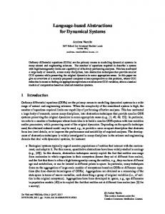
I. I NTRODUCTION Embedded systems are typically controlled by software that conceptually manipulates real-valued quantities, for instance measurements of environment data. Such quantities are stored in a computer as floating-point numbers. As only few real numbers can be encoded in this format, values must generally be rounded to some nearby floating-point number. Compared to a computation with infinite precision, rounding can influence program behavior in multiple ways. The deviation caused by rounding can lead to unintuitive results, such as in a non-associative addition operation. Worse, the deviation can accumulate and eventually change the control flow of the program. Implementations of floating-point algorithms can be sensitive to very small variations in input. Bugs caused by such rounding errors are therefore often hard to reproduce and to test for, and have been referred to as “Heisenbugs” [1]. If undetected, they can have tragic consequences, as embedded devices are used in many mobile and ubiquitous computing environments. A prominent example is the Ariane 5 disaster, caused by an out-of-bounds 64-bit floating-point conversion. The indisputable need for reliability in embedded applications calls for precise and rigorous formal analysis methods. Programs with floating-point arithmetic have been addressed in the past in various ways. In abstract interpretation [2], the program is (partially) executed on an abstract domain, such as real intervals. The generated transformations may, however, turn out too coarse for definite decisions on the given properties. Proof assistants are tools that prove theorems about programs (involving floating-point arithmetic) under human guidance. This guide, unfortunately, must be highly skilled to direct the tool towards a proof. Both abstract interpretation and theorem proving often lack the ability to generate This research is supported by the the Toyota Motor Corporation, by the Semiconductor Research Corporation (SRC) under contract no. 2006-TJ-1539, by the EU FP7 STREP MOGENTES (project ID ICT-216679), and by the EPSRC project EP/G026254/1.
counterexamples for invalid properties, which is essential for debugging and for the high-impact field of automated testvector generation. In this paper, we present a precise and sound decision procedure for (binary) floating-point arithmetic for the automatic analysis of software. A principal way of achieving this is to encode floating-point operations as functions on bit-vectors, and relying on efficient solvers for bit-vector logic, for instance those based on “bit-flattening” and subsequent SAT-solving. Unfortunately, this approach has proven to be intractable in practice, simply because it results in very large and hard-tosolve SAT instances, as we will illustrate. A common solution to address this problem is to use approximations of formulas. Particularly, an overapproximation φ simplifies the formula φ in a way that preserves all satisfying assignments; thus, unsatisfiability of φ implies unsatisfiability of φ. Analogously, an underapproximation φ simplifies φ in a way that removes satisfying assignments; thus, any satisfying assignment to φ can be adjusted to one for φ. Classical counterexample-guided abstraction refinement (CEGAR) [3] relies on overapproximations, which are refined if spurious counterexamples (in the form of spurious satisfying assignments) are encountered. In [4], a decision procedure for bit-vector arithmetic is presented that employs both types of approximations, although in a fixed alternation schedule. Such approaches are too rigid for floating-point arithmetic, as some formulas do not permit effective overapproximations, while others do not permit effective underapproximations. In this paper, we propose a new abstraction method for checking the satisfiability of a floating-point formula φ. Our algorithm permits a mixed sequence S of both over- and underapproximating transformations. The formula ψ resulting from applying S to φ is in general neither an over- nor an underapproximation of φ. Our algorithm stops whenever (i) the simplified formula ψ permits a satisfying assignment that satisfies φ, too, or (ii) ψ is unsatisfiable and permits a resolution proof that is also a valid proof for φ. If neither of the opportunities (i) and (ii) applies, S needs to be refined. If ψ was found to be spuriously satisfiable, the algorithm removes an overapproximating transformation from S, otherwise an underapproximating transformation. Our algorithm can be seen as a framework for a class of abstraction-based procedures to check the satisfiability of formulas in some logic: different choices of the transformation sequence S result in different instances of our framework. For example, the work presented in [4] is an instance where S strictly alternates between over- and underapproximations.
CEGAR is an instance where S contains only overapproximations. Our paper generalizes these methods in a way that permits a choice of approximations based on their effectiveness to simplify the input formula. Termination of any algorithm based on our framework is guaranteed as long as the sequence S can be shown to be depleted eventually. We demonstrate the utility of the procedure on decision problems arising in bounded model checking (BMC) [5] of ANSI-C programs. II. P RELIMINARIES : F LOATING -P OINT A RITHMETIC A. The IEEE floating-point format The binary floating-point format is used to represent real numbers in a computer. Specifically, the triple consisting of a sign s ∈ {0, 1}, an integer-valued exponent e, and a rational-valued mantissa m represents the floating-point number (−1)s · m · 2e . According to the IEEE standard 754, the three components are encoded using bit-vectors, resulting in the partitioned representation of a floating-point number shown in Figure 1. s ←→
er−1 · · · e0 ←−−−−−−−−−−→
mp−1 · · · m0 ←−−−−−−−−−−−−−→
1
r
p
Fig. 1.
The three fields of an IEEE-754 floating-point number
The sign bit s directly represents the sign of the floatingpoint number. The following two bit-vector fields are interpreted as follows: • The bit field e ¯ := er−1 . . . e0 encodes the integral exponent e as a binary number. • Together with the hidden bit, the bit field m ¯ := mp−1 . . . m0 encodes the fractional value of the mantissa m; the representation ensures that 0 ≤ m < 2. The hidden bit is derived from e¯, and is used to distinguish normal and denormal numbers. The widths r and p of the second and third bit fields in Figure 1 are called the range and the precision of the representation. The IEEE standard 754 defines two types of floating-point numbers: the single format with (r, p) = (8, 23), and the double format with (r, p) = (11, 52). Unrepresentable real numbers are rounded, as we review in Section II-B. Numbers that are too large are represented using the symbols −∞ and +∞. The floating-point number NaN (“Not a Number”) represents results of operations outside of real arithmetic, such as imaginary values. We call the floatingpoint numbers ±∞ and NaN special; they are represented using reserved patterns for exponent and mantissa. In this paper, we manipulate floating-point formulas by varying the precision parameter p, while parameter r is fixed. We denote by Fp the set consisting of the floating-point numbers (−1)s ·m·2e representable as a bit-vector with precision p, and the special numbers ±∞. With R∞ := R ∪ {±∞}, we have −∞ ≤ x ≤ +∞ for all x ∈ R∞ . Obviously, for p0 ≤ p, we have Fp0 ⊆ Fp ⊂ R∞ .
B. Floating-point arithmetic The result of an operation a ◦ b, for ◦ ∈ {+, −, ×, /}, may not be representable in Fp even though a and b are in Fp .1 In such a case, an appropriate approximation is selected. For x ∈ R, define the approximations bxcp and dxep as bxcp
:=
max{f ∈ Fp : f ≤ x} ,
dxep
:=
min{f ∈ Fp : f ≥ x} .
and
The values bxcp and dxep are the two floating-point numbers in Fp nearest to x. There is no floating-point number strictly between bxcp and dxep . If x is larger than any non-special floating-point number in Fp , then dxep = +∞; analogously for bxcp . The approximation values satisfy the following nesting property: for p0 ≤ p, bxcp0 ≤ bxcp ≤ x ≤ dxep ≤ dxep0 . Definition 1: A rounding function is a function rd p : R → Fp such that, for all x ∈ R, rd p (x) ∈ {bxcp , dxep }. Specific rounding functions are also known as rounding modes. Two examples of rounding modes are round-up (rd p = d·ep ) and round-down (rd p = b·cp ). The floating-point operators } ∈ {⊕, , ⊗, �} are defined as the rounded result of the corresponding real operators ◦ ∈ {+, −, ×, /}: Definition 2: For a given rounding function rd p and an arithmetic operation ◦ : R2 → R, the corresponding floatingpoint operation }p : F2p → Fp is defined by x }p y := rd p (x ◦ y) . The IEEE standard 754 extends this definition to operations with special operands, e.g. +∞⊕p −∞ := NaN. Note that, due to the rounding, associativity does not hold for floating-point operations, i.e., (a }p b) }p c may differ from a }p (b }p c). Floating-point arithmetic (FPA) (with precision p) is the logic defined by the structure hFp , =, ≤, }i. A term is an expression over arithmetic operations involving variables or constants over Fp . We also allow conversions between terms with different precision. Given terms t1 , t2 , atoms in FPA are of the form t1 ./ t2 with ./ ∈ {=, ≤}. The Boolean connectives ∧, ∨, ¬ are used to construct formulas. We consider the combination of FPA with integer bit-vector arithmetic (BVA) and allow both semantic and bit-wise conversions between integer bit-vectors and floating-point bit-vectors. The goal of this work is a decision procedure that determines the satisfiability of FPA+BVA formulas. III. P ROPOSITIONAL E NCODINGS OF FPA F ORMULAS Given a circuit implementation of an IEEE-754 compliant floating-point unit (FPU), each floating-point operation can be modeled as a formula in propositional logic, as we illustrate below. This way, a formula in FPA can — in principle — be translated to an equisatisfiable formula in propositional logic and passed to a SAT-solver to check for satisfiability. This suggests a sound and complete decision procedure for FPA. 1 For instance, the addition of the binary numbers 1.1 · 20 ∈ F and 1 1.0 · 20 ∈ F1 (1 bit fractional precision) results in 10.1 · 20 , which is not representable with 1 bit fractional precision and a mantissa m < 2.
er
High-level overview of a floating-point adder/subtracter.
A LIGN. The mantissa of the smaller operand is shifted by |ea − eb | bits to the right, rendering the two exponents equal. • A DD /S UB . The two resulting mantissas are then added, resp. subtracted, with a standard integer adder. • ROUND . If the new mantissa has more than p bits, the result is rounded to obtain a number in Fp . The rounding is implemented as a function on the least significant bits of the mantissa. If ea = eb = es = er , the A LIGN module is not needed, since the shift distance is 0. The ROUND module can also be simplified, since the mantissa is not shifted. In this case, the circuit implements fixed-point arithmetic: the operation is reduced to the A DD /S UB module. The existence of efficient SAT-encodings for fixed-point arithmetic formulas therefore suggests that reducing the cost of the A LIGN and ROUND modules may improve the performance of a floating-point decision procedure via a SAT-encoding. Table I shows the number of propositional variables needed for a floating-point adder/subtracter (optimized for propositional SAT, not area or depth), depending on the width p of the mantissa. These numbers confirm that alignment and rounding •
Precision p=5 p = 11 p = 17 p = 23 p = 29 p = 35 p = 41 p = 47 p = 52
ea eb
rd
sr
A LIGN 295 418 561 687 813 996 1140 1284 1404
A DD /S UB 168 252 336 420 504 588 672 756 826
ROUND 572 853 1153 1447 1744 2050 2362 2665 2923
Total 1035 1523 2050 2554 3061 3634 4174 4705 5153
TABLE I N UMBER OF VARIABLES FOR AN FP- ADDER DEPENDING ON p
div sa ma sb mb Fig. 3.
em mm sm
mr
ROUND
mr
M UL /D IV
Fig. 2.
ROUND
m0a m0b s0a s0b
es ms ss
sub
A LIGN
ma ea sa mb eb sb
A DD /S UB
Figure 2 shows a high-level description of a floating-point adder/subtracter as implemented in most FPUs. An adder/subtracter is composed of three modules.
B. Multiplication and division A high-level description of a floating-point multiplier/divider is given in Figure 3. Besides the rounder as described above, an FPU implements the following modules for a multiplier/divider: • A DD /S UB . The exponents of the two operands are first added, for multiplication, resp. subtracted, for division. • M UL /D IV . The two mantissa are then multiplied, resp. divided.
er sr
rd
A. Addition and Subtraction
cause the propositional formula to blow up in size. One way to curb this blow-up is to approximate floating-point operations by reducing the precision p, as we shall do in Section IV.
A DD /S UB
The bottleneck is of course the complexity of the resulting propositional formulas, as we demonstrate in the following. Our analysis also hints at sources for approximating these formulas in meaningful ways.
High-level overview of a floating-point multiplier/divider
Table II shows the number of propositional variables needed for a floating-point multiplier/divider, depending on the width p of the mantissa. As one would expect, the multiplier/divider Precision p=5 p = 11 p = 17 p = 23 p = 29 p = 35 p = 41 p = 47 p = 52
M UL /D IV 280 982 2188 3898 6112 8830 12052 15778 19268
A DD /S UB 94 94 94 94 94 94 94 94 94
ROUND 674 1287 1910 2258 3200 3855 4521 5193 5742
Total 1048 2363 4192 6550 9406 12779 16667 21065 25104
TABLE II N UMBER OF VARIABLES FOR AN FP- MULTIPLIER DEPENDING ON p
yields a propositional formula that is expensive to decide. One possibility to curb these costs is to reduce the precision p, as this reduces the width of the multiplier. We now discuss how formulas are approximated when p is reduced. IV. A PPROXIMATING F LOATING -P OINT A RITHMETIC Reducing the precision of floating-point operations approximates the input formula: a satisfiable formula may become unsatisfiable, or vice versa. In order for the results returned by a SAT solver to still be useful, we need to be aware of the “direction” of the approximation. In this section, we discuss methods for over- and underapproximating floatingpoint formulas by reducing their precision.
A. Overapproximation 0
Reducing the precision p of a floating-point operation to p causes the bits needed for the correct rounding decision to be lost, and the rounding to be based on higher-order bits. It turns out that by making the reduced-precision rounding decision nondeterministic, the reduced-precision formula overapproximates the original. Definition 3: The open rounding operation rdp,p0 : P(R) → P(Fp ) is defined as rdp,p0 (X) := [ bXcp0 , dXep0 ] ∩ Fp , where bXcp0 := minx∈X bxcp0 and dXep0 := maxx∈X dxep0 . The set rdp,p0 (X) can be seen as the smallest precisionp floating-point “interval” Y such that for all x ∈ X, the reduced-precision values bxcp0 , dxep0 are in Y . We use the operator rdp,p0 to define corresponding open floating-point operations. Definition 4: For an arithmetic operation ◦ : R2 → R, the corresponding open floating-point operation }p,p0 : (P(Fp ))2 → P(Fp ) is defined as: X }p,p0 Y := rdp,p0 ({x ◦ y | x ∈ X, y ∈ Y }) . The new floating-point operation }p,p0 overapproximates the original operation }p in the sense that }p,p0 yields more results than }p , i.e., x }p y ∈ {x} }p,p0 {y}, for any reduced precision p0 ≤ p, as the following lemma shows. Lemma 1: For p, p0 with p0 ≤ p, x }p y ∈ {x} }p,p0 {y}. Proof: By the definitions of }p and rd p , x}p y = rd p (x◦ y) ∈ {bx ◦ ycp , dx ◦ yep }. We estimate this set as follows: ... ⊆ ⊆ = =
[ bx ◦ ycp , dx ◦ yep ] [ bx ◦ ycp0 , dx ◦ yep0 ] rdp,p0 ({x ◦ y}) {x}}p,p0 {y} .
∩ Fp [closed interval] ∩ Fp [nesting prop.] [Def. 3 with X = {x ◦ y}] [Def. 4]
One can use the open operations to generate a formula φ that overapproximates the original φ. Each floating-point operation }p is replaced by an open version }p,p0 , for some reduced precision p0 . The reduced precision can be chosen separately for each occurrence of a floating-point operation. B. Underapproximation To generate an underapproximation, we devise floatingpoint operations with fewer results than the original operations. Observe that if a floating-point operation with reduced precision p0 yields an exact result, then the same result is obtained with the original precision p. Our new floating-point operations are restricted to exact precision p0 results. To formalize this idea, we define a modified rounding operator rdp,p0 : Definition 5: The no-rounding operator rdp,p0 : P(R) → P(Fp ) is defined as rdp,p0 (X) := X ∩ Fp0 . The quantity rdp,p0 ({x}) equals {x} if no rounding is required to represent x with precision p0 , i.e., x ∈ Fp0 , and the empty
set otherwise, independently of p. Floating-point operations }p,p0 that yield exact results only are defined in analogy to Def. 4, with rd replaced by rd. These operations yield fewer results than their original counterparts }p . That is, if {z} is the result of the new exact operation {x}}p,p0 {y}, then z is also the result of original operation x }p y: Lemma 2: For p, p0 with p0 ≤ p, {x}}p,p0 {y} = {z} implies x }p y = z. Proof: We have {x}}p,p0 {y} = {x◦y}∩Fp0 = {z}, thus z = x ◦ y ∈ Fp0 ⊆ Fp . From x ◦ y ∈ Fp , we can conclude bx ◦ ycp = dx ◦ yep = x ◦ y = rd p (x ◦ y) = x }p y = z. One can use } to generate an underapproximation of a formula φ, by replacing each floating-point operation with a version that is exact for some reduced precision p0 . In case the constructed underapproximation is shown to be unsatisfiable, nothing can be concluded on the satisfiability of φ. One way to resolve the dichotomy between over- and underapproximations is to integrate both into an abstractionrefinement framework. V. T HE M IXED A BSTRACTION F RAMEWORK A. Overview In Section IV, we have presented over- and underapproximation techniques to simplify a given floating-point formula φ. Many existing procedures build either over- or underapproximations, depending on whether the goal is to show satisfiability or unsatisfiability. The two types of approximation guarantee a definite decision on the satisfiability of φ only in cases that are orthogonal for the two types. We therefore propose to combine them in a concerted effort towards analyzing φ. To this end, we propose the abstraction framework shown in Figure 4, which checks the satisfiability of the input formula φ. We first identify a set of eligible transformations. A transformation is a mapping that turns a FPA formula β into a new one that over- or underapproximates β, for example by replacing some floating-point operation by its open version, as suggested in Section IV. The set of transformations is accordingly partitioned into subsets Over and Under . At the beginning of the loop indicated in the figure, an implementation selects some of the eligible transformations and applies them to φ in a particular order. Note that the resulting formula ψ in general neither over- nor underapproximates φ (hence called “mixed”). Exit points of the loop. Formula ψ is then subject to a satisfiability check. Depending on the outcome of this check, the loop can be exited — with a definite answer — if: (i) ψ is satisfiable, and the assignment α returned by the solver (suitably extended) satisfies φ as well. In this case, the overall answer is “SAT”. Or: (ii) ψ is unsatisfiable, and the resolution proof P returned by the solver is valid for φ, too. In this case, the overall answer is “UNSAT”. Refinement. If neither case (i) or (ii) applies, the approximation needs to be refined. This is done by removing some transformations from Over if ψ was found to be spuriously satisfiable, otherwise from Under . Which transformations to
φ Identify eligible transformations Over and Under
Select transformations from Over ∪ Under and apply them to φ ψ Satisfiable ? n yes α) (proo o . fP g s ) (as
α satisfies φ ? no Over := Over \ {o}
Fig. 4.
yes SAT,α
a suitable well-quasi-order on the set of all approximation transformations. The Mixed Abstraction framework generalizes several other abstraction-refinement approaches to satisfiability-checking a formula. The classical CEGAR paradigm conservatively abstract–check–refine can be seen as an instance of Figure 4 where the set Under is empty. Therefore, the test whether an unsatisfiability proof for ψ is valid for φ can be skipped in favor of an immediate answer “UNSAT”. The method presented in [4] has the property that the sequence of approximations obtained from φ strictly alternates between strict over- and strict underapproximations. As we experimentally compare this alternating scheme to our own implementation of mixed abstraction, we sketch first how the method of [4] can be applied in a floating-point environment. VI. I MPLEMENTING M IXED A BSTRACTIONS
proof P valid for φ
? yes UNSAT,P
no Under := Under \ {u}
The Framework of Mixed Abstraction
select for removal is an important implementation decision, which we discuss below in Section VI-B. The loop in Figure 4 is then reentered, and some transformations from the new sets Over and Under are applied to φ. Notice that the procedure can be implemented in a both incremental and backtrackable fashion, provided the underlying SAT solver is incremental and backtrackable. Property 1: Given a formula φ, any algorithm that implements the framework in Figure 4, starting with finite sets Over and Under of transformations, terminates and returns “SAT” if φ is satisfiable, “UNSAT” otherwise. Proof: (a) Partial correctness: The algorithm outputs “SAT” only in the case that the assignment α was validated successfully against the original formula φ. It outputs “UNSAT” only in the case that an unsatisfiability proof for ψ was found to be a valid proof of unsatisfiability for φ. (b) Termination: In each round in which the algorithm does not exit, at least one element is removed from Over or from Under . When both sets are exhausted, ψ and φ are equivalent, and one of the two exit conditions is trivially satisfied. Note that the correctness property is independent of the distribution and scheduling of over- and underapproximations, and of the strategy for selecting elements o or u to remove in each iteration. Furthermore, it can be shown that finiteness of the sets Over and Under is not even required if one defines
A. Alternating Abstractions for Floating-Point Arithmetic The alternating approach by Bryant et al. [4] to integrating over- and underapproximations was implemented for integer bit-vector arithmetic formulas. If the SAT-check on an approximated formula is inconclusive, information obtained from the SAT checker is used to generate a refined approximation of the opposite type, and the procedure repeats. We can use the approximation methods presented in Section IV to apply the alternating approach to floating-point arithmetic, as follows. We begin with an overapproximation φ of φ. To obtain φ, the transformations in Over replace all floating-point operations } by }p,p0 , for some initial reduced precision p0 . Since Under is not applied, φ is an overapproximation. If φ is unsatisfiable the procedure terminates. Otherwise, the decision procedure yields an assignment α. If α also satisfies φ, the procedure halts and returns α as a witness. If α is spurious, we extract from it the operands a, b, and the result r of each occurrence of }p,p0 . In case r 6= }p we conclude that r is a spurious result and we refine (increase) the precision of }p0 ; otherwise p0 is left unchanged. Next, the decision procedure builds a refined underapproximation φ as explained in Section IV-B. In this iteration, the transformations in Under replace all occurrences of } by }p,p0 for the refined precisions p0 ; no transformation from Over is applied. In case φ is satisfiable, the procedure terminates and returns α as an assignment for φ. Otherwise, the decision procedure yields an UNSAT proof P for φ. If P is also a proof for φ, the procedure halts and returns P . Otherwise, it checks whether the constraint X ∩ Fp of an exact operation }p0 (Definition 5) is contained in P . If it is, the precision is increased; otherwise it is left unchanged. The next iteration constructs a refined overapproximation. Altogether, this yields a sound and complete decision procedure alternating between over- and underapproximations. The problem with this approach is that the alternating schedule of over- and underapproximations often leads to ineffective approximations, as some formulas are not amenable to effective overapproximations, while others do not permit
effective underapproximations. As an example, consider the non-associativity formula (a⊕b)⊕c 6= a⊕(b⊕c). This formula is satisfiable, as floating-point addition ⊕ is not associative. Satisfiability cannot be proved using an overapproximation. On the other hand, every strict underapproximation of this formula turns out to be unsatisfiable. Thus, this formula cannot be decided using either strict over- or strict underapproximations. Our experimental results (Section VII) confirm these predictions for realistic formulas. The lesson is that an implementation of Mixed Abstraction should not be “forced” to apply either type of abstraction for pure schedule reasons. Instead, the structure of the formula itself should dictate how to approximate it. This leads to our approach of “genuinely mixed abstractions”, which we present in the following. B. Genuinely Mixed Abstractions We now detail our implementation of the mixed abstraction framework. The selection of abstractions is determined by the structure of the formula, and which approximations are most effective on it. We begin with both a very coarse overapproximation and a strong underapproximation: the result of the operation is completely nondeterministic and forced to zero at the same time. Depending on the outcome of the satisfiability check of ψ, either one of these approximations is refined, gradually lifting constraints or gradually increasing the precision of the operator. The simulation of α on φ in the left branch in Figure 4 can be preceded by a check whether any transformation in Over was applied to φ. If not, ψ is guaranteed to be an underapproximation of φ, and “SAT” and α are returned immediately. Otherwise, α is suitably extended to an assignment for φ and checked for satisfaction of φ, as suggested by the figure. A simple and efficient pre-check whether an unsatisfiability proof P for ψ is extendable to φ can be performed by computing the set Var (P ) ∩ Var (Under ). This set contains the variables occurring in (the clauses of) the proof P that are involved in any of the underapproximation transformations in Under . If empty, we conclude that the underapproximation transformations applied to φ are not responsible for the unsatisfiability result for ψ, which hence applies to φ, too. The emptiness test can obviously be optimized by checking first whether any transformation in Under was applied to φ. If none of the exit tests succeeds, the algorithm selects approximation transformations o or u to remove at the end of the loop body, in order to refine the approximation. Let us look first at the case that ψ was found to be satisfiable, but the assignment α is spurious (does not satisfy φ). If there exists a transformation o ∈ Over such that α does not satisfy the formula obtained by simplifying φ using all transformations except o, we can select such an o: its removal guarantees that the spurious assignment α disappears in the next round. If there is no such transformation, we select some o that affects the variables occurring in the spurious assignment α. If ψ was found to be unsatisfiable, the algorithm computes the set Var (P ) ∩ Var (Under ), as discussed above. If this set is non-empty, then there exists at least one u ∈ Under such
that Var (u) ∩ Var (Under ) is non-empty. The algorithm picks such an element u for removal from Under . After refining the sets Over and Under as described, Figure 4 suggests to apply the refined (and smaller) sequence of approximations to φ again. In practice, approximations selected for removal in the previous step are revoked, so that only local modifications to ψ are necessary. This allows the subsequent satisfiability check to be done incrementally, without restarts of the SAT solver. VII. E XPERIMENTAL R ESULTS A. Implementation and Benchmarks We have implemented the algorithm proposed in this paper in combination with a standard bit-flattening decision procedure for integer bit-vector arithmetic. The procedure supports all operators required to model ANSI-C programs. The procedure is fully incremental: the clauses for those parts of the encoding that are not modified, and any clauses learned from those, are retained between iterations. We use MiniSAT2 [6] as our SAT solver. The performance of the integer bit-vector decision procedure we use is comparable to that of a state-of-the-art SMT-BV solver. The benchmarks we use are derived from a variety of publicly-available C programs, selected from the SNU realtime [7] and the Mediabench benchmarks [8]; the programs we have selected make extensive use of single- or doubleprecision floating-point arithmetic. Our encoding is able to support changes of the rounding mode during the program execution, as the rounding mode may be set separately for each individual operator in the formula. However, none of the benchmark programs makes use of this feature, and we have used “round to nearest even” uniformly. We have not observed a significant impact of the specific rounding mode on the performance of either the full encoding or the abstractionrefinement procedure. In order to obtain verification conditions, we have manually annotated our benchmarks with properties in the form of arithmetic assertions; a few of the programs already contain some (light-weight) assertions. The main property we check is the possibility of arithmetic exceptions, as defined in the IEEE floating-point arithmetic standard. These properties turn out to be difficult; an instance of a counterexample is arithmetic underflowing to zero and a subsequent division of two such numbers, which results in NaN. Such counterexamples can only be obtained if encoding artifacts such as denormal numbers are modelled in a precise manner. After the annotation, we pass the programs to CBMC [9], which generates a total of 119 FPA decision problems. A satisfying assignment for such a formula corresponds to a counterexample that demonstrates that an assertion can be violated. Our experiments were performed on a machine running Linux on an Intel Xeon CPU with 3 GHz and 4 MB cache. B. Results Figure 5 compares the runtime of the mixed abstraction with the full flattening, for a timeout of 1000 s and a memory
Mixed Abstraction
1000 100 10 1 0.1 0.1
Fig. 5.
1 10 100 1000 Without Abstraction
Runtime comparison of full flattening and the mixed abstraction
limit of 2 GB. The mixed abstraction is not dominating; in some cases (6 out of 119), the final abstraction contains almost all operators at full precision, and as a result, the immediate full flattening is faster. On the other hand, there are 58 large instances for which the abstraction-refinement procedure terminates within the timeout, whereas the full flattening aborts due to excessive memory consumption. Let us look at some benchmarks in more detail. For a timeout of 7 hours, Table III provides a comparison of the performance of three methods: the full flattening, an alternating abstraction as proposed in [4], and the mixed abstraction. The entries illustrate particular weaknesses and strengths of the three procedures. First of all, even small programs may result in decision problems that are simply too large (or too hard) for a full flattening. Similarly, there are instances in which the alternating abstraction is unable to proceed beyond the first iteration, as either the pure under- or overapproximation is already too hard. The mixed abstraction terminates on a number of instances that are too hard for the other procedures, but typically requires a large number of iterations. This is owed to the extremely coarse initial abstraction, combining both over- and underapproximations. As long as the intermediate abstractions are solvable, the alternating abstraction may converge quicker to a solution (e.g., consider sqrt.c, claim 2). VIII. R ELATED WORK A popular approach to verifying software with floating-point operations is to use proof assistants, i.e., programs that prove theorems under the guidance of a human expert. A variety of assistants have been used to prove upper bounds for the deviation from the real arithmetic result of a calculation. Examples include proofs using HOL [10], HOL-Light [11]– [13] and ACL2 [14], [15]. However, in case no proof is found, proof assistants typically return little evidence as to whether the proof goal was actually invalid, or whether the proof strategy was too weak to establish its validity. An alternative approach is to use abstract interpretation [2] together with domains that can soundly approximate floatingpoint computations for classical static analysis. The static ´ [16] uses a number of domains which analyzer ASTREE
can soundly abstract floating-point computations, including intervals, octagons, polyhedra, and ellipsoid domains. The adaptation of abstract domains for floating-point numbers is a non-trivial problem due to issues of rounding, the possibility of overflows and underflows, and division by zero errors. Relational abstract domains such as the octagon domain rely on associativity and distributivity of arithmetic operations. These properties do not hold for floating-point ´ floating-point expressions are therefore numbers. In ASTREE, approximated by linear expressions over the real field with interval coefficients [17] before they are transformed into their target abstract domains. In [18], a floating-point polyhedra abstract domain based on these ideas is presented. Their linearisation technique is implemented in the APRON library for static analysis [19], which provides sound handling of floating-point expressions for a number of abstract domains. The propagation of floating-point rounding errors has also been studied extensively in the framework of abstract interpretation [20]–[23]. Such analyses allow to quantify deviations of floating-point computations from their exact result in arithmetic over the reals. Verifying floating-point programs using abstract interpretation shares with our method the advantage of being fully automatic. However, in case the property does not hold, it is usually difficult to obtain a counterexample that can be reproduced on the actual program. Neither interactive theorem provers nor the use of abstract domains enjoy the characteristics of a decision procedure, namely completeness and full automation in deciding floatingpoint expressions. There has been some work on decision procedures for floating-point arithmetic in the field of constraint satisfaction programming (CSP). Solvers for CSP instances containing floating-point constraints have been applied to automated test-vector generation [24], [25]. This approach combines filtering the possible values of variables using interval techniques with a search procedure for finding actual floating-point values inside these intervals. Their algorithm is mainly geared towards test-vector generation, not verification. The authors state that in some cases where the calculated intervals overapproximate the concrete variable values too coarsely, their approach is unable to terminate with an answer in reasonable time. This includes the case where no such concrete solutions exist. In this paper, we are interested in verification of software using floating-computations. A different, but related field of research is the verification of floating-point hardware. The work described in [26] is an example of such an approach and provides an overview over the relevant literature. IX. C ONCLUSION We have presented an algorithm for iteratively approximating a complex formula by mixing both under- and overapproximations to obtain a formula ψ. In contrast to prior work, ψ need not be an over- nor an underapproximation and can therefore be constructed in a way that yields formulas that are easy to solve. Experimental results indicate improved
Benchmark qurt.c, qurt.c, qurt.c, qurt.c, qurt.c, qurt.c, qurt.c, sqrt.c, sqrt.c, minver.c, minver.c, sin.c, sin.c, sin.c, gaussian.c,
claim claim claim claim claim claim claim claim claim claim claim claim claim claim claim
1 2 3 4 5 6 7 1 2 1 2 1 2 3 1
Lines of Code 109 109 109 109 109 109 109 51 51 156 156 46 46 46 108
Satisfiable? no no no no no no no no yes no yes no no no no
No Abstr. time (s) 25 25 25 OM 25 25 6716 24 9 1 2 13864 13831 TO TO
Alternating [4] time (s) #iter. 15 1 15 1 15 1 OM 1 15 1 15 1 OM 1 TO 3 608 2 1 1 2 2 1892 1 1894 1 TO 3 TO 1
Mixed time (s) #iter. 2 15 0.6 7 1 13 478 103 1.2 15 0.6 7 84 86 13589 44 TO 107 0.1 1 0.1 1 281 47 281 47 1074 63 14437 137
TABLE III C OMPARISON OF F ULL F LATTENING TO A LTERNATING AND M IXED A BSTRACTION
robustness compared to a plain flattening and to an abstractionrefinement scheme based on an alternation of over- and underapproximations. The algorithm supports incremental solving, is complete, and produces witnesses. In particular, the ability to generate counterexamples for invalid specifications is essential not only for debugging, but also for the high-impact field of automated test-vector generation, where counterexamples to carefully crafted specifications translate into test cases meeting certain coverage criteria. One aspect of future work is how to vary the exponent width r in order to approximate a floating-point operation. While the operations on the exponent contribute only the smaller part of the propositional encoding, many programs exist that only exercise a very small range of exponent values. R EFERENCES [1] Gander, W.: Heisenberg effects in computer-arithmetic (2005) http:// www.inf.ethz.ch/news/focus/res focus/april 2005. [2] Cousot, P., Cousot, R.: Abstract interpretation: a unified lattice model for static analysis of programs by construction or approximation of fixpoints. In: Principles of Programming Languages (POPL). (1977) 238–252 [3] Clarke, E.M., Grumberg, O., Jha, S., Lu, Y., Veith, H.: Counterexampleguided abstraction refinement. In: Computer Aided Verification (CAV). (2000) 154–169 [4] Bryant, R.E., Kroening, D., Ouaknine, J., Seshia, S.A., Strichman, O., Brady, B.A.: Deciding bit-vector arithmetic with abstraction. In: Tools and Algorithms for the Construction and Analysis of Systems (TACAS). (2007) 358–372 [5] Biere, A., Cimatti, A., Clarke, E.M., Strichman, O., Zhu, Y.: Bounded model checking. Advances in Computers 58 (2003) 118–149 [6] E´en, N., S¨orensson, N.: An extensible SAT-solver. In: Theory and Applications of Satisfiability Testing (SAT). (2003) 502–518 [7] SNU Computer Architecture and Network Laboratory: SNU Real-Time Benchmarks. (1995) http://archi.snu.ac.kr/realtime/benchmark. [8] Lee, C., Potkonjak, M., Mangione-Smith, W.H.: Mediabench: A tool for evaluating and synthesizing multimedia and communicatons systems. In: International Symposium on Microarchit (MICRO). (1997) 330–335 [9] Clarke, E.M., Kroening, D., Lerda, F.: A tool for checking ANSI-C programs. In: Tools and Algorithms for the Construction and Analysis of Systems (TACAS). (2004) 168–176 [10] Carreno, V.A.: Interpretation of IEEE-854 floating-point standard and definition in the HOL system. Technical report, NASA Langley Research Center (1995)
[11] Harrison, J.: Formal verification of square root algorithms. Form. Methods Syst. Des. 22 (2003) 143–153 [12] Harrison, J.: Formal verification of floating point trigonometric functions. In: Formal Methods in Computer-Aided Design (FMCAD). (2000) 217–233 [13] Harrison, J.: Floating point verification in HOL light: The exponential function. In: Algebraic Methodology and Software Technology (AMAST). (1997) 246–260 [14] Russinoff, D.M.: A mechanically checked proof of correctness of the AMD K5 floating point square root microcode. Form. Methods Syst. Des. 14 (1999) 75–125 [15] Russinoff, D.M.: A case study in fomal verification of register-transfer logic with ACL2: The floating point adder of the AMD AthlonTM processor. In: Formal Methods in Computer-Aided Design (FMCAD). (2000) 3–36 [16] Blanchet, B., Cousot, P., Cousot, R., Feret, J., Mauborgne, L., Min´e, A., Monniaux, D., Rival, X.: A static analyzer for large safety-critical software. In: Programming Language Design and Implementation (PLDI). (2003) 196–207 [17] Min´e, A.: Relational abstract domains for the detection of floating-point run-time errors. In: European Symposium on Programming (ESOP). (2004) 3–17 [18] Chen, L., Min´e, A., Cousot, P.: A sound floating-point polyhedra abstract domain. In: Asian Symposium on Programming Languages and Systems (APLAS). (2008) 3–18 [19] Jeannet, B., Min´e, A.: APRON: A library of numerical abstract domains for static analysis. In: Computer Aided Verification (CAV). (2009, to appear) [20] Goubault, E.: Static analyses of the precision of floating-point operations. In: Static Analysis (SAS). (2001) 234–259 [21] Goubault, E., Martel, M., Putot, S.: Asserting the precision of floatingpoint computations: A simple abstract interpreter. In: European Symposium on Programming (ESOP). (2002) 209–212 [22] Martel, M.: Static analysis of the numerical stability of loops. In: Static Analysis (SAS). (2002) 133–150 [23] Putot, S., Goubault, E., Martel, M.: Static analysis-based validation of floating-point computations. In: Numerical Software with Result Verification. (2003) 306–313 [24] Michel, C., Rueher, M., Lebbah, Y.: Solving constraints over floatingpoint numbers. In: Principles and Practice of Constraint Programming (CP). (2001) 524–538 [25] Botella, B., Gotlieb, A., Michel, C.: Symbolic execution of floatingpoint computations. Softw. Test., Verif. Reliab. 16 (2006) 97–121 [26] Jacobi, C., Berg, C.: Formal verification of the VAMP floating point unit. Formal Methods in System Design 26 (2005) 227–266