Information Sciences and Computing Volume 2015, Article ID ISC490415, 21 pages Available online at http://www.infoscicomp.com/
Research Article
Mixed Curvelet and Wavelet Transforms for Speckle Noise Reduction in Ultrasonic B-Mode Images A.A. Mahmouda, S. El Rabaiea, T.E. Tahaa, O. Zahrana, F.E. Abd El-Samiea and W. AlNauimyb a
Department of Electronics and Electrical Communications, Faculty of Electronic Engineering, Menoufia University, 32952, Menouf , Egypt b Department of Electrical Engineering and Electronics at the University of Liverpool, UK Corresponding author: A.A. Mahmoud; E-mail:
[email protected] Received 21 November 2014; Accepted 17 January 2015
Abstract: Wavelet transform has the good characteristic of time-frequency locality and many researches show that it can perform well for denoising in smooth and singular areas. But it isn’t suitable for describing the signals, which have high dimensional singularities. Curvelet is one of new multiscale transform theories, which possess directionality and anisotropy, and it breaks some inherent limitations of wavelet in representing directions of edges in image. So it has superiority in some image analysis, such as image denoising. This paper proposes a new method for denoising, which combines Curvelet transform and wavelet transform which is better than only using wavelet transform or Curvelet transform to deal with noisy image. The simulation results indicate that this method has better performance and can get better visual effects and higher PSNR.
Keywords: Image enhancement; Ultrasonic scan; Speckle noise; Denoising filters.
1. Introduction Ultrasound imaging, as a tool for medical diagnosis, is widely used in clinical practice, and in some situation sit has become a standard procedure. Although diagnostic ultrasound is considered a harmless technique and permits real-time and noninvasive anatomical scanning, B-mode images are pervaded by the speckle artifact, which results from destructive interference effects between returning echoes. This artifact introduces fine-false structures whose apparent resolution is beyond the capabilities of the imaging system, reducing image contrast and masking the real boundaries of the tissue under investigation. Its occurrence may substantially compromise the diagnostic effectiveness, introducing a great level of subjectivity in the interpretation of the images [1- 3].
Information Sciences and Computing
2
Speckle can be defined as a destructive interference artifact and its severity depends on the relative phase between two overlapping returning echoes. Like other imaging techniques that make use of coherent sources, such as laser or radar, images from ultrasound acoustical waves are prone to speckle corruption that should be removed without affecting the important details in the image [1, 2]. This paper is organized as follows. Section 2 gives details about Log Gabor filter in the Wavelet domain. Section 3 illustrates the Curvelet transform. Section 4 explains the proposed approach. Section 5 proposes the simulation results followed by conclusions and the more relevant references.
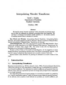
2. Log Gabor Filter in the Wavelet Domain 2.1 Discrete Wavelet Transform (DWT) The idea of the DWT is to represent an image as a series of approximations (low pass version) and details (high pass version) at different resolutions. The image is low pass filtered to give an approximation image and high pass filtered to give detail images, which represent the information lost when going from a higher resolution to a lower resolution. Then the wavelet representation is the set of detail coefficients at all resolutions and approximation coefficients at the lowest resolution. Figure (1): (a) shows the operation of two dimensional DWT with 3-Level decomposition and (b) shows the operation of a single step decomposion-reconstruction DWT [4- 7]. An input series is processed by two filters in parallel. h1(n) is called low pass filter (or average filter) and h2(n) is high pass filter (or difference filter). The outputs obtained are then down sampled by two so that now both the outputs are half of original length. After the first step of processing on the original series, a new series is formed with the output of the low pass filter forming the first half and the output of the high pass filter forming the second half.
Figure (1-a): 2D-DWT with 3-Level decomposition
Information Sciences and Computing
3
Figure (1-b): One level of wavelet decomposition and reconstruction The matrix of the DWT has four subbands (LL, LH, HL, HH), the subband LL, the approximate, is the low resolution part and the subbands LH, HL, HH, the details, are the high resolution part. In the next step, only the first half of the new series that is the output of the low pass filter is processed. This kind of processing and new series formation continues till in the last step the outputs obtained from both the filters are of length one. The original length of the series needs to be a power of two so that the process of DWT can be carried until the last step [4- 7]. The approximate image and the detail image can be expressed as follows: Y 1 (n ) =
Y 2 (n ) =
∞
∑
k = −∞ ∞
∑
k = −∞
X ( k ) h1 (2 n − k )
X ( k ) h 2 (2 n − k ) (1)
Where h1 is low pass filter and h2 is the high pass filter. A Haar wavelet is the simplest wavelet type. In discrete form, Haar wavelet is related to a mathematical operation called the haar transform. The Haar transform serves as a prototype for all other wavelet transforms. The Haar decomposition has good time localization. This means that the Haar coefficients are effective for locating jump discontinuities and also for the efficient representation of images with small support. The Haar wavelet is the only known wavelet that is compactly supported, orthogonal and symmetric. It is computed by iterating difference and averaging between odd and even samples of the signal. Since we are in 2D, we need to compute the average and difference in the horizontal and then in the vertical direction [6, 8, 9].
2.2 Log Gabor Filter Images are better coded by filters that have Gaussian transfer functions when viewed on the logarithmic frequency scale. Gabor functions have Gaussian transfer functions when viewed on the linear frequency scale. On the linear frequency scale the LogGabor function has a transfer function of the form:
Information Sciences and Computing
=
⁄ ⁄
4
(2)
Where f0 is the filter centre frequency and σ/f0 is the ratio of the standard deviation of the Gaussian describing the log Gabor filter's transfer function in the frequency domain to the filter center frequency. There are two important characteristics to note. Firstly, log-Gabor functions, by definition, always have no DC component, and secondly, the transfer function of the log Gabor function has an extended tail at the high frequency end [10- 13].
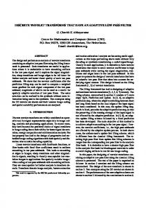
3. Curvelet Transform The wavelet transform has been the most famous tool for image and signal analysis. This is because of its advantageous property that helps to localize “point singularities” in the signal or the image. One major disadvantage of wavelets in image processing is that the two-dimensional wavelet transform gives a large number of coefficients in all scales (across all levels) corresponding to the edges of the image. This means that many coefficients are required in order to exactly reconstruct the edges in an image. Recent approaches like Ridgelets and Curvelets exploit the fact that wavelets are good only for point singularities but not efficient to handle linear and curvilinear singularities in an image. The Curvelet transform provides sparsity and effective representation of edges or singularities [14, 15]. The Ridgelet transform is implemented by applying a one-dimensional wavelet transform to the slices of the Radon transform. The Ridgelet transform alone cannot yield efficient representations of images, because edges in images are typically curved rather than straight lines. Therefore, the approach to capture curved edges is to use Ridgelets in a localized manner such that a curved edge is almost a straight line at sufficiently fine scales. The Ridgelet transform is then extended to Curvelet transform which gives a more efficient representation of curved lines in an image than using only the Ridgelet transform. It has to be noted that both the Ridgelet and Curvelet transforms are based on the Radon transform [15, 16]. In Curvelet transforms, the additive wavelet transform is used to decompose the image into different subbands and partitioning is used to break each subband into tiles. Finally, the Ridgelet transform is applied to each tile. In this way, the image edges can be represented efficiently by the Ridgelet transform because the image edges will now be almost like straight lines. Thus, the Curvelet transform is an extension of the Ridgelet transform to detect curved edges, effectively [14- 19]. The Curvelet map the curvilinear structures effectively in an image by using the anisotropic scale space approach considering a curvilinear edge as piecewise linear segments across different scales. The mapping of the edges using Curvelets is shown diagrammatically in the Fig. 5.1. Curvelets apply the Ridgelet transform locally in order to obtain the localization information. The continuous line shown is a typical curved edge and the dotted straight lines are the approximate mapping of the curved edge. Since the Ridgelet transform is efficient for linear edges, the curved edge is approximated as linear segments. The blocking or the partitioning step of the Curvelet transform achieves this segmentation of the curved edge [15].
Information Sciences and Computing
5
Figure 2: The curvelet map curvilinear edges in image as piecewise Ridgelets Ridgele in sufficiently fine scales. The continuous line shows the edge in the image and the dotted lines show the corresponding map as piecewise linear ridges The algorithm of the curvelet transform can be summarized in the following steps [14, [ 19]: ∆ ∆ 1. The image is split up into three subbands 1 , 2 and P3 using the additive wavelet transform. ∆ ∆ 2. Tiling is performed on the subbands 1 and 2 . 3. The discrete Ridgelet transform is performed on each tile of the subbands ∆1 and
∆2
.
A schematic diagram of the curvelet transform is depicted in Figure 3. 3 A detailed description of these steps is presented in the following subsections.
Figure 3: Schematic diagram of the discrete curvelett transform. transform
3.1 Sub Band Filtering The purpose of this step is to decompose the image into additive components each of which hich is a subband of the image. This step isolates the different frequency components of the image into different planes without down sampling as in the
Information Sciences and Computing
6
traditional wavelet transform. The "`a trous" algorithm given below is implemented for this purpose [14, 19]. The "`a trous" algorithm is shift invariant, symmetric, undecimated and redundant DWT algorithm that is widely used in image analysis. In order to understand the "`a trous" algorithm, it is very useful to represent the wavelet transform as a parallelepiped. The basis of the parallelepiped is the original image 2j; each level of the parallelepiped is an approximation to the original image. When climbing up through the resolution levels, the successive approximation images have a coarser resolution but the same number of pixels as the original image [15]. Given an image p , it is possible to construct the sequence of approximations [14]: f 1 ( p ) = p1, f 2 ( p1 ) = p 2 , f 3 ( p 2 ) = p3,…, f n ( p n −1 ) = pn
(3)
To construct this sequence, the algorithm performs successive convolutions with a filter associated with the scaling function. A popular choice for the corresponding scaling function is the triangle function which leads to a linear interpolation with a 3 mask of 3x3 elements. For a B - spline scaling function, the coefficients of the mask are [14]: 1 4 6 4 1 4 16 24 16 4 1 6 24 36 24 6 256 4 16 24 16 4 1 4 6 4 1 (4) The wavelet planes are computed as the differences between two consecutive approximations Pl −1 and Pl [14], i.e.,
(
w l = Pl −1 − Pl l = 1,2,............., n
)
(5)
Thus, the reconstruction formula is given by [14]: n
P = ∑w l + Pr l =1
(6)
Where Pr is the residual image that contains the low frequency information of the original image, and wl its respective wavelet coefficients, which contain the high frequency information. The next step is finding a transformation capable of representing straight edges with different slopes and orientations. A possible solution is the Ridgelet transform, which may be interpreted as the 1-D wavelet transform of the Radon transform. This is the basic idea behind the digital implementation of the Ridgelet transform. An inconvenience with the Ridgelet transform is that it is not capable of representing curves. To overcome this drawback, the input image is partitioned into square blocks
Information Sciences and Computing
7
and the Ridgelet transform is applied to each block. Assuming a piecewise linear model for the contour, each block will contain straight edges only, that may be analyzed by the Ridgelet transform.
3.2 Tiling Tiling is the process by which the image is divided into overlapping tiles. These tiles are small in dimensions to transform curved lines into small straight lines in the ∆ ∆ subbands 1 and 2 [14, 19]. The tiling improves the ability of the curvelet transform to handle curved edges.
3.3 Ridgelet Transform The motivation for this transform arose from a need to find a sparse representation of functions which have discontinuities along lines. We choose the Ridgelet transform because the wavelet transform is very efficient in representing point discontinuities in the 1-D case, but fails with edge discontinuities in 2-D case. The Ridgelet transform is not better than the wavelet transform in representing edges in 2-D [14, 16, 20]. The Ridgelet transform belongs to the family of discrete transforms employing basis functions. To facilitate its mathematical representation, it can be viewed as a wavelet analysis in the Radon domain. The Radon transform itself is a tool for shape detection. So, the Ridgelet transform is primarily a tool for ridge detection or shape detection of the objects in an image [14- 16, 19, 20].
3.3.1 Continuous Ridgelet Transform 2 The 2-D continuous Ridgelet transform in R can be defined through the introduction of the following basis function [14, 17, 20]:
ψ a ,b ,θ = a −1/2ψ
( x 1 cosθ + x 2 sinθ −b ) a
(7)
Where a indexes the scale of the Ridgelets, θ its orientation and b , its location. For θ ∈ ( 0, 2π ) each a > 0 , each b ∈ R and each . Thus, the Ridgelet coefficients are represented by [14, 17, 20]: R f (a,b ,θ ) =
∞ ∞
∫ ∫ ψ a,b ,θ (x 1, x 2 )f (x 1, x 2 )dx 1dx 2 −∞ −∞
(8)
This transform is invertible and the reconstruction formula is given by [14, 20]: f (x 1, x 2 ) =
2π ∞ ∞
da
dθ
∫0 −∞∫ ∫0 R f (a,b ,θ )ψ a ,b ,θ (x 1, x 2 ) a3 db 4π
The Radon transform for an object f is given by [14, 17, 20]:
(9)
Information Sciences and Computing
Rf (θ ,t ) =
8
∞ ∞
∫ ∫ f ( x 1, x 2 )δ ( x 1 cosθ + x 2 sinθ −t )dx 1dx 2 −∞ −∞
(10)
Thus, the Ridgelet transform can be represented as follows [14, [ 17, 20]: ]: R f (a,b ,θ ) =
∞
∫ Rf (θ ,t )a −∞
ψ (t − b ) dt
−1/2
a
(11)
Hence, the Ridgelet transform is the application of a 1-D 1 D wavelet transform to the slices of the Radon transform where the angular variable θ is constant and t is varying. A schematic diagram of the Ridgelet transform is shown in Figure Fig 4. To make the Ridgelet transform discrete both the Radon transform and the wavelet transform have to be discrete [14, [ 17, 19].
Figure 4: Schematic diagram agram of the Ridgelet transform 3.3.1.1 Radon Transform The Radon transform is a fundamental tool which is used in various applications such as radar imaging, geophysical imaging and medical imaging. It is used to detect features within a 2-D D image. It transforms lines through an image to points in the Radon domain as shown in Figure Fig 5. In the Radon back projection, each point in the Radon domain is transformed to a straight line in the image [14[ 18].
Figure 5: The Radon Transform.
Information Sciences and Computing
9
The Radon transform for an object f is the collection of line integrals indexed by (θ , t ) ∈ [ 0, 2π ] × R (integral of the function on the straight line L passing through t and of direction θ ) and is expressed using Dirac mass δ given by [14- 18]: Rf (θ ,t ) =
∞ ∞
∫ ∫ f ( x 1, x 2 )δ ( x 1 cosθ + x 2 sin θ − t )dx 1dx 2 −∞ −∞
(12)
3.3.2 Digital Ridgelet Transform A basic strategy for calculating the continuous Ridgelet transform is first to compute the Radon transform Rf (θ , t ) and second, to apply a 1-D wavelet transform. For practical applications, we require discrete implementations of the Ridgelet transform that is a challenging problem, since the Radon transform is polar in nature, we cannot implement direct discretizations of continuous formulae. Digital Ridgelet has been proposed, based on implementation of the Radon transform [16]. 3.3.2.1 The Recto Polar Ridgelet Transform Approximate Radon transforms for digital data can be proposed in the Fourier domain, this is a widely used approach. First the two-dimensional fast Fourier transform (2D FFT) of the given image is computed. Then, the resulting function in the frequency domain is to be used to evaluate the frequency values in a pseudo-polar style. This conversion from Cartesian to Polar grid could be obtained by interpolation. Applying the one dimensional inverse Fourier transform for each ray, the Radon projections are obtained [15- 17]. For our implementation of the Cartesian-to-polar conversion, we have used a pseudo polar grid, in which the pseudo-radial variable has level sets which are squares rather than circles. This grid has often been called the concentric squares grid in the signal processing literature. In the medical tomography literature, it is associated with the linogram, sometimes called the rectopolar grid. The geometry of the rectopolar grid is illustrated on Figure 6. [15-17]. Concentric circles of linearly growing radius in the polar grid are replaced by concentric squares of linearly growing sides. The rays are spread uniformly not in angle but in slope. We select 2n radial lines in the frequency plane obtained by k ,k connecting the origin to the vertices ( 1 2 ) lying on the boundary of the array ( k 1 , k 2 ) , i.e., such that k 1 or k 2 ∈{− n 2 , n 2} . The polar grid is the intersection between the set of radial lines and that of Cartesian lines parallel to the axes. The 2 cardinality of the rectopolar grid is equal to 2n as there are 2n radial lines and n sampled values on each of these lines. As a result, data structures associated with this grid will have a rectangular format [15- 17].
Information Sciences and Computing
10
pseudo polar grid in the frequency domain for an n by n Figure 6: Illustration of the pseudo-polar image (n = 8) From the 2- D discrete Fourier expression, we get [16]: [ n −1 n −1
F (w 1 ,w 2 ) = ∑ ∑ f j =1 k =1
( j , k )e
(
− i k w 1 + jw 2
)
(13)
We can change this expression to polar coordinates coordina by: w 1 = ζ cos θ and w 2 = ζ sin θ
Then,
we
replace
2π m , m = 0,....., M − 1 θm = M
in
( (13)
n −1 n −1
F (n , m ) = ∑ ∑ f j =1 k =1
by
( j , k )e
sampling
ζn =
n , n = 0,....., N − 1 N
− i n k cos 2π m + j sin 2π m N M M
and
(14)
To obtain samples ples on the rectopolar grid, we should, in general, interpolate from nearby samples at the Cartesian grid. 3.3.2.2 One-Dimensional Dimensional Wavelet Transform To complete the Ridgelet transform, we must take a 1-D 1 D wavelet transform transfo along the radial variable in Radon space. Figure 7. shows the flow graph of the Ridgelet transform [16- 19].
Information Sciences and Computing
11
Figure 7:: Discrete Ridgelet Transform flow graph
4. Curvelet Denoising Algorithm We now apply a digital transforms for removing removing speckle noise from ultrasonic image data. The methodology is based on the work published in [16]. [ ]. Unlike FFTs or FWTs, discrete curvelet transform is not norm-preserving norm preserving and, therefore, the variance of the noisy curvelet coefficients will depend on the t curvelet index λ. Let Yλ be the noisy curvelet coefficients (Y ( = FX). ). We use the following hardhard thresholding rule for estimating the unknown curvelet coefficients
yˆ λ = y λ,
if y λ / σ ≥ k σˆλ
yˆ λ = 0, if y λ / σ < k σˆλ
(15)
Where For the first scale (j=1) a scale-dependent scale value alue k = 4 was chosen; while k = 3 for the others (j > 1).
5. The Proposed Approach The Proposed approach depends on the combining the advantages of both the Wavelet and Curvelet transform. The proposed approach can be summarized in the following steps: 1. 2. 3. 4.
The noisy image is split into three subbands C1, C2 and P3 using DCT, as explained. Wavelet transform of the subband P3. Log Gabor filtering of the Wavelet subbands except the approximate. Inverse Wavelet transform of the filtered subbands and the approximate. approx
Information Sciences and Computing
5.
12
Hard thresholding of the subbands C1 and C2 and Inverse Discrete Curvelet Transform (IDCT).
6. Simulation Results Computer simulations were carried out using MATLAB (R2007b). The quality of the reconstructed image is specified in terms of: The Peak Signal-to-Noise Ratio (PSNR) [21]: =
(16)
Where MSE, the Mean Square Error between the estimate of the image and the original image, and !" # is the maximum possible pixel value in the image. The Coefficient of Correlation (CoC): $ $=
∑' ∑)&
./∑' ∑)
+ ',) *+ , ',) *,
+ 0 ',) *+ 0/∑' ∑) , ',) *,
(17)
Here x (m, n) is the pixel intensity or the gray scale value at a point (m, n) in the undeformed image. y (m, n) is the gray scale value at a point (m, n) in the deformed + are mean values of the intensity matrices x and y, respectively. image. + and , Simulation results are conducted on six examples of ultrasonic B-mode images (Liver, Kidney, Fetus, Thyroid, Breast and Gall) [22]. The Proposed approach for ultrasonic image denoising is applied to the six examples (Liver, Kidney, Fetus, Thyroid, Breast and Gall) images. Results are compared to the DCT algorithm results. The first example (Liver image) is shown in Fig. (8-a), the 0.1 speckle noisy image is shown in Fig. (8-b), the DCT output image is shown in Fig. (8-c) and the proposed approach output image is shown in Fig. (8-d). The second example (Kidney image), shown in Fig. (9-a), the 0.1 speckle noisy image is shown in Fig. (9-b), the DCT output image is shown in Fig. (9-c) and the proposed approach output image is shown in Fig. (9-d). The same for the third example (Fetus image), shown in Fig. (10-a), the 0.1 speckle noisy image is shown in Fig. (10-b), the DCT output image is shown in Fig. (10-c) and the proposed approach output image is shown in Fig. (10-d). The fourth example (Thyroid image), shown in Fig. (11-a), the 0.1 speckle noisy image is shown in Fig. (11-b), the DCT output image is shown in Fig. (11-c) and the proposed approach output image is shown in Fig. (11-d).
Information Sciences and Computing
13
The fifth example (Breast image), shown in Fig. (12-a), the 0.1 speckle noisy image is shown in Fig. (12-b), the DCT output image is shown in Fig. (12-c) and the proposed approach output image is shown in Fig. (12-d). The last example (Gall image), shown in Fig. (13-a), the 0.1 speckle noisy image is shown in Fig. (13-b), the DCT output image is shown in Fig. (13-c) and the proposed approach output image is shown in Fig. (13-d). Tables from (1) to (6) illustrate the output PSNR values for the proposed approach and the DCT for the six examples, respectively, with (0.01, 0.05, 0.1 and 0.2) speckle variances. Tables from (7) to (12) illustrate the output CoC values for the proposed approach and the DCT for the six examples, respectively, with (0.01, 0.05, 0.1 and 0.2) speckle variances. Table (13) illustrates the output CPU time (sec) considerations for the proposed approach and the DCT for the six examples.
(a) Original Liver image
(b) 0.1 speckle noisy image
(c) DCT denoised output image
(d) The Proposed approach output image
Figure 8: Proposed approach and DCT output images for the Liver image
(a) Original Kidney image
(b) 0.1 speckle noisy image
(c) DCT denoised output image
(d) The proposed approach output image
Figure 9: Proposed approach and DCT output images for the Kidney image
Information Sciences and Computing
(a) Original Fetus image
(b) 0.1 speckle noisy image
14
(c) DCT denoised output image
(d) The proposed approach output image
Figure 10: Proposed approach and DCT output for the Fetus image
(a) Original Thyroid image
(b) 0.1 speckle noisy image
(c) DCT denoised output image
(d) The proposed approach output image
Figure 11: Proposed approach and DCT output for the Thyroid image
(a) Original Breast image.
(b) 0.1 speckle noisy image.
(c) DCT denoised output image.
(d) The proposed approach output image.
Figure 12: Proposed approach and DCT output for the Breast image
Information Sciences and Computing
(a) Original Gall image.
(b) 0.1 speckle noisy image.
15
(c) DCT denoised output image.
(d) The proposed approach output image.
Figure 13: Proposed approach and DCT output for the Gall image
Table 1: PSNR output values for the proposed approach and DCT denoising algorithm for the first example at speckle variance of (0.01: 0.2) The first example (Liver image) Noise variance 0.01
0.05
0.1
0.2
PSNR Noisy
31.51
25.97
23.92
22.04
PSNR DCT
33.64
30.44
29.09
27.51
PSNR proposed
33.74
30.50
28.89
27.96
Table 2: PSNR output values for the proposed approach and DCT denoising algorithm for the second example at speckle variance of (0.01: 0.2) The second example (Kidney image) Noise variance 0.01
0.05
0.1
0.2
PSNR Noisy
23.03
20.52
18.42
16.60
PSNR DCT
28.68
25.90
24.98
23.98
PSNR proposed
28.71
25.97
24.96
24.01
Information Sciences and Computing
16
Table 3: PSNR output values for the proposed approach and DCT denoising algorithm for the third example at speckle variance of (0.01: 0.2) The third example (Fetus image) Noise variance 0.01
0.05
0.1
0.2
PSNR Noisy
29.54
23.98
21.94
20.16
PSNR DCT
34.62
30.70
28.87
27.06
PSNR proposed
34.60
30.32
29.20
27.59
Table 4: PSNR output values for the proposed approach and DCT denoising algorithm for the fourth example at speckle variance of (0.01: 0.2) The fourth example (Thyroid image) Noise variance 0.01
0.05
0.1
0.2
PSNR Noisy
29.19
24.14
21.73
20.09
PSNR DCT
33.85
29.52
27.73
27.06
PSNR proposed
33.50
29.84
27.88
27.29
Table 5: PSNR output values for the proposed approach and DCT denoising algorithm for the fifth example at speckle variance of (0.01: 0.2) The fifth example (Breast image) Noise variance 0.01
0.05
0.1
0.2
PSNR Noisy
30.28
24.99
22.38
20.83
PSNR DCT
32.20
29.26
27.29
25.80
PSNR proposed
32.44
28.42
27.08
25.60
Information Sciences and Computing
17
Table 6: PSNR output values for the proposed approach and DCT denoising algorithm for the sixth example at speckle variance of (0.01: 0.2) The sixth example (Gall image) Noise variance 0.01
0.05
0.1
0.2
PSNR Noisy
30.40
24.65
22.54
20.72
PSNR DCT
33.27
29.50
27.97
25.88
PSNR proposed
33.39
29.10
27.60
25.91
Table 7: CoC output values for the proposed approach and DCT denoising algorithm for the first example at speckle variance of (0.01: 0.2) The first example (Liver image) Noise variance 0.01
0.05
0.1
0.2
CoC Noisy
0.9817
0.9172
0.8523
0.7550
CoC
DCT
0.9894
0.9731
0.9599
0.9396
proposed
0.9897
0.9735
0.9603
0.9402
CoC
Table 8: CoC output values for the proposed approach and DCT denoising algorithm for the second example at speckle variance of (0.01: 0.2) The second example (Kidney image) Noise variance 0.01
0.05
0.1
0.2
CoC Noisy
0.9792
0.9076
0.8393
0.7303
CoC DCT
0.9891
0.9728
0.9597
0.9390
0.9896
0.9730
0.9604
0.9399
CoC
proposed
Information Sciences and Computing
18
Table 9: CoC output values for the proposed approach and DCT denoising algorithm for the third example at speckle variance of (0.01: 0.2) The third example (Fetus image) Noise variance 0.01
0.05
0.1
0.2
CoC Noisy
0.9813
0.9154
0.8496
0.7565
CoC DCT
0.9941
0.9801
0.9649
0.9384
0.9939
0.9798
0.9654
0.9409
CoC
proposed
Table 10: CoC output values for the proposed approach and DCT denoising algorithm for the fourth example at speckle variance of (0.01: 0.2) The fourth example (Thyroid image) Noise variance 0.01
0.05
0.1
0.2
CoC Noisy
0.9655
0.8591
0.7609
0.6366
CoC DCT
0.9869
0.9671
0.9515
0.9284
0.9870
0.9668
0.9503
0.9286
CoC
proposed
Table 11: CoC output values for the proposed approach and DCT denoising algorithm for the fifth example at speckle variance of (0.01: 0.2) The fifth example (Breast image) Noise variance 0.01
0.05
0.1
0.2
CoC Noisy
0.9835
0.9243
0.8645
0.7738
CoC DCT
0.9894
0.9691
0.9488
0.9113
0.9893
0.9691
0.9461
0.9140
CoC
proposed
Information Sciences and Computing
19
Table 12: CoC output values for the proposed approach and DCT denoising algorithm for the sixth example at speckle variance of (0.01: 0.2) The sixth example (Gall image) Noise variance 0.01
0.05
0.1
0.2
CoC Noisy
0.9849
0.9297
0.8755
0.7875
CoC DCT
0.9926
0.9749
0.9568
0.9379
0.9924
0.9743
0.9539
0.9389
CoC
proposed
Table 13: CPU time output values for the proposed approach and DCT denoising algorithm for the six examples The six examples
CPU DCT CPU proposed
Liver
Kidney
Fetus
Thyroid
Breast
Gall
159.77
168.92
150.44
150.11
161.85
150.61
169.25
174.47
167.06
168.58
165.22
170.07
As can be seen in the proposed approach output images, speckle is greatly reduced as compared to the original images. Also, preservation of most the structure of the original ultrasonic image is apparent. The proposed approach significantly reduces the speckle noise while preserving the resolution and the structure of the original ultrasonic images. The wavelet transform handles smooth and singular areas very well but it has some problem with edges. On the other hand, hard thresholding in the curvelet domain handles edges very well but has some problem when dealing with smooth and singular areas. By combining the wavelet transform and the curvelet transform, as is done in this chapter, by letting wavelet transform handles homogeneous areas while curvelet transform handles areas with edges we get optimized results. The proposed approach gives good, clean and high contrast images, which should improve medical diagnosis.
7. Conclusion This paper presents an approach depends on the combining the advantages of both the Wavelet and Curvelet transform. Wavelet transform can perform well for denoising in smooth and singular areas but it has not optional base when dealing with singular line
Information Sciences and Computing
20
and surface. Curvelet transform breaks some inherent limitations of Wavelet in representing directions of edges in image. So it has superiority in some image analysis, such as image denoising so it is better to combines Curvelet transform and wavelet transform which is better than only using wavelet transform or Curvelet transform to deal with noisy image. Output images and PSNR values indicate superior performance over only Wavelet or Curvelet.
References [1] [2] [3] [4]
[5]
[6]
[7] [8] [9] [10]
[11] [12]
[13] [14] [15] [16] [17] [18]
[19]
R.G. Dantas and E.T. Costa, Ultrasound speckle reduction using modified gabor filters, IEEE Trans., Ultrason., Ferroelectr., Freq. Control, 54(2007), 530-538. C.B. Burckhardt, Speckle in ultrasound b-mode scans, IEEE Trans. Sonics Ultrason., 25(1) (1978), 1-6. R.F. Wagner, S.W. Smith, J.M. Sandrik and H. Lopez, Statistics of speckle in ultrasound B-scans, IEEE Trans., Sonics Ultrason., 30(3) (May) (1983), 156-163. L. Kaur, S. Gupta and R.C. Chauhan, Image denoising using wavelet thresholding, Third Conference on Computer Vision, Graphics and Image Processing, India, December 16-18 (2002). S.K. Mohideen, S.A. Perumal and M.M. Sathik, Image denoising using discrete wavelet transform, International Journal of Computer Science and Network Security, 8(1) (January) (2008), 213-216. N. Jacob and A. Martin, Image denoising in the wavelet domain using wiener filtering, Unpublished Course Project, University of Wisconsin, Madison, Wisconsin, USA, (2004). V. Strela, Denoising via block wiener filtering in wavelet domain, 3rd European Congress of Mathematics, Barcelona, Birkhäuser Verlag, July (2000). J. Cook, V. Chandran and S. Sridharan, Multiscale representation for 3-d face recognition, IEEE Trans. on Information Forensics and Security, (2007). D.L. Donoho and I. Johnstone, Adapting to unknown smoothness via wavelet shrinkage, J. American. Stat. Assoc., 90(1995), 1200-1224. R. Zewail, A. Seil, N. Hamdy and M. Saeb, Iris identification based on log-gabor filtering, Proceedings of the IEEE Midwest Symposium on Circuits, Systems & Computers, 1(December) (2003), 333-336. J. Cook, V. Chandran and S. Sridharan, Multiscale representation for 3-d face recognition, IEEE Trans. on Information Forensics and Security, (2007). A. Karargyris, S. Antani and G. Thoma, Segmenting anatomy in chest x-rays for tuberculosis screening, Engineering in Medicine and Biology Society, EMBC, Annual International Conference of the IEEE, August (2011), 7779-82. P. Kovesi, Phase preserving denoising of images, Proc. DICTA 99 (Perth, Australia), (1999), 212-217. F.E. Ali, I.M. El-Dokany, A.A. Saad and F.E.S. Abd El-Samie, Curvelet fusion of mr and ct images, Progress in Electromagnetics Research C, 3(2008), 215-224. M.J. Fadili and J.L. Starck, Curvelets and Ridgelets, Encyclopedia of Complexity and Systems Science, Meyers, Robert (Ed.), Springer New York, 2007. J.L. Starck, E. Candes and D.L. Donoho, The curvelet transform for image denoising, IEEE Transactions on Image Processing, 11(6) (2002), 670-684. J.L. Starck, E. Candes and D.L. Donoho, Astronomical image representation by the curvelet tansform, Astronomy and Astrophysics, 398(2003), 785-800. M. Choi, R.Y. Kim, M.R. Nam and H.O. Kim, Fusion of multispectral and panchromatic satellite images using the curvelet transform, IEEE Geosci. Remote Sensing Lett., 2(2005), 136-140. B.B. Saevarsson, J.R. Sveinsson and J.A. Benediktsson, Combined wavelet and curvelet denoising of SAR images, Proceedings of IEEE International Geoscience and Remote Sensing Symposium, (IGARSS), 6(2004), 4235-4238.
Information Sciences and Computing
[20] [21] [22]
21
E.J. Candes and D.L. Donoho, Ridgelets: The key to higher-dimensional intermittency? Phil. Trans. R. Soc. Lond. A., 357(1999), 2495-2509. Q. Huynh-Thu and M. Ghanbari, Scope of validity of PSNR in image/video quality assessment, Electronics Letters, 44(13) (2008), 800-801. http://www.google.com.eg/search ultrasonic image, Date of Access 6 December (2011).
Copyright © 2015 A.A. Mahmoud, S. El Rabaie, T.E. Taha, O. Zahran, F.E. Abd El-Samie and W. Al-Nauimy. This is an open access article distributed under the Creative Commons Attribution License, which permits unrestricted use, distribution, and reproduction in any medium, provided the original work is properly cited.