Namely, the transform will take a data set with a more or less flat histogram and produce a data set which has just a few large values and a very high number of ...
Mathematical Geophysics Summer School, Stanford, August 1998
Wavelet transforms and compression of seismic data G. Beylkin
I
1
and A. Vassiliou
2
Introduction
Seismic data compression (as it exists today) is a version of transform coding which involves three main steps: 1. The transform step, which is accomplished by a fast wavelet, wavelet-packet or local cosine transform; 2. The quantization step, which is typically accomplished by a scalar uniform or non-uniform quantization scheme, and 3. The encoding step, which is accomplished by entropy coding such as Huffman coding or adaptive arithmetic coding. Let us briefly outline the role of each step. The role of the transform step is to decorrelate the data. Namely, the transform will take a data set with a more or less flat histogram and produce a data set which has just a few large values and a very high number of near zero or zero values. In short, this step prepares the data for quantization. It has been observed that a much better compression is achieved by quantizing the decorrelated data than the original data. There are several transforms that can be used for decorrelation. For example, the Karhunen-Loeve transform achieves decorrelation but at a very high computational cost. It turns out that the wavelet, wavelet-packet or local cosine transforms can be used instead. These transforms are fast and provide a local time-scale (or time-frequency) data representation, resulting in a relatively few large coefficients and a large number of small coefficients. At the second step the coefficients of transformed data are quantized, i.e., mapped to a discrete data set. The quantization can take two forms, either scalar quantization, or vector quantization. In the case of scalar quantization every transform coefficent is quantized separately whereas in the case of vector quantization a block of coefficients is quantized simultaneously. Based on practical experience with seismic data it appears that the transformed coefficents tend to be reasonably decorrelated, thus pointing to scalar quantization as a good option. The most straightforward type of scalar quantization is uniform quantization, where the range of the coefficient values is divided into intervals of equal lehgth (bins), except possibly for a separate bin near zero (zero bin). Since the quantization step is the only lossy step of the process, a certain level of optimization has to take place in order to accommodate the target compression ratio (or the target bit budget). 1
Department of Applied Mathematics, University of Colorado at Boulder, Boulder, CO 80309-0526 and Fast Mathematical Algorithms and Hardware, 1020 Sherman Avenue, Hamden, CT 06514 2 GeoEnergy Corporation, 2530 East 71 Street, Suite E, Tulsa, OK 74136
1
A distortion criterion (implied by the size of the seismic gather or ensemble of gathers and the target compression ratio) is minimized subject to the bit budget. In some cases a non-uniform quantization can yield lower distortion level than the uniform quantization. We note that some new quantization/coding schemes which have been used for image compression may not be directly applicable to seismic data. For example, embedded zerowavelet tree compression (EZW) scheme [13] does not appear efficient since seismic data violate the basic assumptions of EZW algorithm. After quantization we are likely to have a number of repeated quantized coefficients and, thus, a significant redundancy. The third step, entropy coding, addresses this issue. Perhaps the easiest analogy to entropy coding comes from the Morse code communication, in which frequently encountered symbols are transmitted with shorter codes, while rarely encountered symbols are transmitted with longer codes. The entropy coding creates a new data set which has the average number of bits/sample minimized. There are two distinct cases of entropy coding. In the case of stationary data one can use Huffman coding. In the case of non-stationary data adaptive arithmetic coding is usually applied. Now that we have an overall picture, we will desribe individual steps in greater detail. The notions that are considered below are not yet a familiar territory for a geophysicist and, for that reason, our goal will be limited to providing a basic trail map. We will consider the basic steps in the reverse order so that it is clear (at least intuitively) what is desirable to have as an output of the preceding step.
II
Entropy coding
Let us consider a finite set of symbols S = (x 1 , x2 , . . . , xN ). Let pn denote the propability of P occurence of the symbol xn in some set X (elements of which are from S), N n=1 pn = 1. Let us associate a binary word wn of length ln with each symbol xn . By aggregating binary words, we produce a code for X. The average bit rate in order to code X is RX =
N X
ln pn .
n=1
It makes sense to select short code words w n for symbols with high propability so to minimize RX . It is important to note that we should be able to identify the binary words uniquely from their “aggregated state”. This can be achieved by using the so-called prefix codes where short binary words do not occur as the beginning of longer binary words. Such codes are constructed using binary trees where words correspond to the leaves of the tree. The binary digits of the code words are obtained by using 0 and 1 to correspond to left and right branches of the tree along the path to the node. Thus, the number of binary digits corresponds to the depth of the tree for a given node. Shannon’s theorem provides the lower bound for the average bit rate R X , namely, the entropy H(X) = −
N X
n=1
pn log2 pn ≤ RX . 2
The Huffman algorithm (Huffman coding) [7] constructs an optimal prefix tree and the corresponding code so that H(X) ≤ RX ≤ H(X) + 1. The difficulty in obtaining the lower bound via Huffman coding is that it requires l n = − log2 pn and log2 pn generally is not an integer. In order to avoid this constrain the algorithm of arithmetic coding [16] codes a sequence of symbols. The average bit rate of arithmetic coding approaches asymptotically the lower bound and in practice performes somewhat better than Huffman coding. Finally, we note that probabilities of symbols are typically computed from N most recent symbols. This quick overview should make it clear that the role of Steps 1 and 2 is to provide to entropy coder a set with a minimal number of symbols where very few of the symbols carry “most of the probability”.
III
Quantization
An example of quantization is analog-to-digital converter with a fixed number of bits (say 24 bits). Clearly quantization is a lossy procedure by its nature. In this sense the digital data (e.g., seismogram) is already quantized. We are seeking a more efficient quantization. The result of quantization is a set X of symbols (e.g., real numbers) that serves as an input to entropy coding. In general, quantization proceeds by taking the interval of variation of the signal and decomposing it into subintervals (called quantization bins). The center of the quantization bin can serve as a symbol (the standard round-off is an example here). The uniform quantizer is a special case where all bins are of the same length. A nonuniform quantizer uses bins of different size. Another way to visualize quantization is to consider a grid on an interval (e.g., centers of the bins) and think of assigning the closest grid point to the real numbers that are being quantized. Further distinction is drawn between scalar and vector quantization. Real numbers can be quantized in groups (vectors) and then one should think of a multidimensional grid corresponding to the multidimensional bins. If one considers quantization and entropy coding together, it is clear that we should try to represent the signal with a minimal number of components, and control the dynamic range and significance of these components. Preparing the data for quantization and entropy coding falls on Step 1. The choice of the transformation is critical for the effective overall compression.
IV
The transform step
The role of the transform step is to separate the more significant “coordinates” (coefficients) from the less significant. Initially one can wonder if such goal can be accoplished without the detailed knowledge of the signal. Indeed, if the usual representation of the signals by their samples were optimal, then very little could have been done without additional information. However, sampled representations are not optimal in any sense: they can be locally oversampled and be overly sensitive to the effects of quantization. 3
Traditionally, the Karhunen-Loeve transform was thought as a method of decorrelating the data. In fact there is a belief that this transform provides the optimal decorrelation. Although there is a theorem with a statement addressing this point (see e.g. [9], Proposition 11.3), it is important to remember that the Karhunen-Loeve transform is optimal for the random Gaussian process. Since this assumption may not be satisfied in practice, one has to be careful in stating optimality of this transformation. In fact it was shown [1] (under an assumption of “piecewise stationary process” for the undelying signals) that the wavelet transform performs better that the Karhunen-Loeve transform. Another problem with the Karhunen-Loeve is its cost. It requires diagonalization of covariance matrix and is too expennsive for using on large data sets. This is where the wavelet transform and its cousins play a very important role.
V
Wavelet Transform
The Haar basis (Haar 1910) [6] provides a simple illustration of wavelet bases. The Haar basis in L2 (R), ψj,k (x) = 2−j/2 ψ(2−j x − k), where j, k ∈ Z, is formed by the dilation and translation of a single function ψ(x) =
1
for 0 < x < 1/2 −1 for 1/2 ≤ x < 1 0 elsewhere.
(5.1)
The Haar function ψ satisfies the two-scale difference equation, ψ(x) = ϕ(2x) − ϕ(2x − 1),
(5.2)
where ϕ(x) is the characteristic function of the interval (0, 1). The characteristic function ϕ(x) is a prototype of the scaling function for wavelets and satisfies the two-scale difference equation, ϕ(x) = ϕ(2x) + ϕ(2x − 1).
(5.3)
Given N = 2n “samples” of a function, which may for simplicity be thought of as values of scaled averages of f on intervals of length 2 −n , s0k
=2
n/2
Z
2−n (k+1)
f (x)dx,
(5.4)
2−n k
we obtain the Haar coefficients as
and averages as
1 dj+1 = √ (sj2k−1 − sj2k ) k 2
(5.5)
1 sj+1 = √ (sj2k−1 + sj2k ) k 2
(5.6)
4
for j = 0, . . . , n − 1 and k = 0, . . . , 2n−j−1 − 1. It is easy to see that evaluating the whole set of coefficients djk , sjk in (5.5), (5.6) requires 2(N − 1) additions and 2N multiplications. In two dimensions, there are two natural ways to construct the Haar basis. The first is simply the tensor product ψj,j 0 ,k,k0 (x, y) = ψj,k (x)ψj 0 ,k0 (y), so that each basis function ψj,j 0 ,k,k0 (x, y) is supported on a rectangle. The second basis is defined by the set of three kinds of basis functions supported on squares: ψ j,k (x)ψj,k0 (y), ψj,k (x)ϕj,k0 (y), and ϕj,k (x)ψj,k0 (y), where ϕ(x) is the characteristic function of the interval (0, 1) and ϕ j,k (x) = 2−j/2 ϕ(2−j x − k). Let us now turn to compactly supported wavelets with vanishing moments constructed in [4], following [10] and [8]. For a complete account we refer to [5]. We start with the definition of the multiresolution analysis. Definition V.1 A multiresolution analysis is a decomposition of the Hilbert space L 2 (Rd ), d ≥ 1, into a chain of closed subspaces . . . ⊂ V2 ⊂ V1 ⊂ V0 ⊂ V−1 ⊂ V−2 ⊂ . . .
(5.7)
such that 1.
T
j∈Z Vj
= {0} and
S
j∈Z Vj
is dense in L2 (Rd )
2. For any f ∈ L2 (Rd ) and any j ∈ Z, f (x) ∈ Vj if and only if f (2x) ∈ Vj−1 3. For any f ∈ L2 (Rd ) and any k ∈ Zd , f (x) ∈ V0 if and only if f (x − k) ∈ V0 4. There exists a function ϕ ∈ V0 such that {ϕ(x − k)}k∈Zd is a Riesz basis of V0 . Let us define the subspaces Wj as an orthogonal complement of Vj in Vj−1 , Vj−1 = Vj ⊕ Wj ,
(5.8)
L2 (Rd ) =
(5.9)
so that M
Wj .
j∈Z
Selecting the coarsest scale n, we may replace the chain of the subspaces (5.7) by Vn ⊂ . . . ⊂ V2 ⊂ V1 ⊂ V0 ⊂ V−1 ⊂ V−2 ⊂ . . . ,
(5.10)
and obtain L2 (Rd ) = Vn
M
Wj .
(5.11)
j≤n
If there is a finite number of scales then without loss of generality we set j = 0 to be the finest scale and consider Vn ⊂ . . . ⊂ V 2 ⊂ V 1 ⊂ V 0 ,
V0 ⊂ L2 (Rd )
instead of (5.10). In numerical realizations the subspace V 0 is finite dimensional. 5
(5.12)
Let us consider a multiresolution analysis for L 2 (R) and let {ψ(x − k)}k∈Z be an orthonormal basis of W0 . We will require that the function ψ has M vanishing moments, Z
+∞
ψ(x)xm dx = 0,
m = 0, . . . , M − 1.
−∞
(5.13)
This property is critical for using wavelet transform as a tool for compression. Property (5.13) implies that the functions which (locally) are well approximated by polynomials have small wavelet coefficients. For the Haar basis M = 1 in (5.13). Are there constructions other than the Haar basis with M > 1? The answer is positive and here we will only show how to derive equations (for the orthonormal case) and refer to [5] for numerous important details. One of the immediate consequences of Definition V.1 is that the function ϕ may be expressed as a linear combination of the basis functions of V −1 . Since the functions {ϕj,k (x) = 2−j/2 ϕ(2−j x − k)}k∈Z form an orthonormal basis of Vj , we have ϕ(x) =
X √ L−1 2 hk ϕ(2x − k).
(5.14)
k=0
In general, the sum in (5.14) does not have to be finite and by choosing a finite sum in (5.14) we are selecting compactly supported wavelets. We may rewrite (5.14) as ϕ(ξ) ˆ = m0 (ξ/2)ϕ(ξ/2), ˆ where
(5.15)
+∞ 1 ϕ(ξ) ˆ =√ ϕ(x) eixξ dx, 2π −∞ and the 2π-periodic function m0 is defined as
Z
m0 (ξ) = 2−1/2
L−1 X
(5.16)
hk eikξ .
(5.17)
k=0
Assuming orthogonality of {ϕ(x − k)} k∈Z , we note that δk0 =
Z
+∞ −∞
ϕ(x − k)ϕ(x) dx =
and, therefore, δk0 =
Z
2π 0
and X l∈Z
X l∈Z
Z
+∞ −∞
2 −ikξ |ϕ(ξ)| ˆ e dξ,
|ϕ(ξ ˆ + 2πl)|2 e−ikξ dξ,
|ϕ(ξ ˆ + 2πl)|2 =
1 . 2π
(5.18)
(5.19)
(5.20)
Using (5.15), we obtain X l∈Z
|m0 (ξ/2 + πl)|2 |ϕ(ξ/2 ˆ + πl)|2 = 6
1 , 2π
(5.21)
and, by taking the sum in (5.21) separately over odd and even indices, we have X
|m0 (ξ/2 + 2πl)|2 |ϕ(ξ/2 ˆ + 2πl)|2
X
|m0 (ξ/2 + 2πl + π)|2 |ϕ(ξ/2 ˆ + 2πl + π)|2 =
l∈Z
+
l∈Z
1 . 2π
(5.22)
Using the 2π-periodicity of the function m 0 and (5.20), we obtain (after replacing ξ/2 by ξ) a necessary condition |m0 (ξ)|2 + |m0 (ξ + π)|2 = 1, (5.23) for the coefficients hk in (5.17). On defining the function ψ by √ X ψ(x) = 2 gk ϕ(2x − k),
(5.24)
k
where gk = (−1)k hL−k−1 ,
k = 0, . . . , L − 1,
(5.25)
or, equivalently, the Fourier transform of ψ by ˆ ψ(ξ) = m1 (ξ/2)ϕ(ξ/2), ˆ where m1 (ξ) = 2−1/2
k=L−1 X k=0
gk eikξ = −e−iξ m0 (ξ + π),
(5.26)
(5.27)
it is not difficult to show, that for each fixed scale j ∈ Z, the wavelets {ψ j,k (x) = 2−j/2 ψ(2−j x− k)}k∈Z form an orthonormal basis of Wj . Equation (5.23) can also be viewed as the condition for exact reconstruction for a pair of the quadrature mirror filters (QMFs) H and G, where H = {h k }k=L−1 and G = {gk }k=L−1 . k=0 k=0 Such exact QMF filters were first introduced by in [14] for subband coding. The decomposition of a function into the wavelet basis is an O(N ) procedure. Given the coefficients s0k , k = 0, 1, . . . , N as “samples” of the function f , the coefficients s jk and djk on scales j ≥ 1 are computed at a cost proportional to N via sjk =
n=L−1 X
j−1 hn sn+2k ,
(5.28)
n=L−1 X
j−1 gn sn+2k .
(5.29)
n=0
and djk
=
n=0
where sjk and djk are viewed as periodic sequences with the period 2 n−j . If the function f is not periodic (e.g. defined on an interval), then such straightforward periodization introduces “artificial” singularities. A better alternative is to use wavelets on the interval [3]. In practice, this approach amounts to modifications near the boundary of both decomposition and reconstruction algorithms. 7
Computing via (5.28) and (5.29) is illustrated by the pyramid scheme {s0k } −→ {s1k } −→ {s2k } −→ {s3k } · · · & & & 1 2 {dk } {dk } {d3k } · · · .
(5.30)
The reconstruction of a function from its wavelet representation is also an order N procedure and is described by j−1 s2n
=
k=M X
h2k sjn−k +
j−1 s2n−1 =
g2k djn−k ,
k=1
k=1
k=M X
k=M X
h2k−1 sjn−k +
(5.31)
k=M X
g2k−1 djn−k .
k=1
k=1
Computing via (5.31) is illustrated by the pyramid scheme {snk } −→ {skn−1 } −→ {skn−2 } −→ {skn−3 } · · · % % % {dkn−1 } {dkn−2 } {dkn−3 } · · · {dnk }
We observe that once the filter H has been chosen, it completely determines the functions ϕ and ψ and, therefore, the multiresolution analysis. Moreover, in properly constructed algorithms, the values of the functions ϕ and ψ are usually never computed. Due to the recursive definition of the wavelet bases, all the manipulations are performed with the quadrature mirror filters H and G, even if they involve quantities associated with ϕ and ψ. As an example, let us compute the moments of the scaling function ϕ, Mm =
Z
xm ϕ(x) dx,
m = 0, . . . , M − 1,
(5.32)
in terms of the filter coefficients {hk }k=L−1 . Applying operator ( 1i d/dξ)m to both sides of (5.15) k=0 and setting ξ = 0, we obtain Mm = 2 where 1
Mhl = 2− 2 Thus, we have from (5.33) Mm
−m
j=m X
m j
j=0
k=L−1 X
hk k l ,
k=0
1 = m 2 −1
j=m−1 X j=0
!
Mj Mhm−j ,
(5.33)
l = 0, . . . , M − 1.
(5.34)
m j
!
Mj Mhm−j ,
(5.35)
with M0 = 1 and we can use (5.35) as a recursion to compute the moments. For the purposes of compression biorthogonal bases are often used [2] but we will not go into details here. 8
VI
What does wavelet transform accomplish?
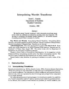
Although the following consideration deals with wavelet transform, similar points can be made for wavelet packets and local trigonometric bases. The coherent portion of the signal in a seismogram appears as a local correlation that our eye easily identifies. Wavelet transform reduces the number of significant coefficients necessary to represent the seismogram locally and, thus, decorrelates the coherent portion of the signal. Vanishing moment are the key to such performance. On the other hand the wavelet transform does not decorelate (or compress) the random Gaussian noise. Thus, the result of application of the wavelet transform is that the coherent portion of the signal will now reside in a relatively few large coefficients whereas the rest of the coefficients will describe a portion of the signal that is like the “random Gaussian noise”. Unfortunately, this heuristics is not precise and there is no theorem asserting the result. Yet, a number of mathematically justified statements are available that indicate that the heuristic picture above is basically correct [1]. For other choices of bases with controlled localization in time-frequency domain similar statements can be made and, in practice, their performance can be somewhat better than that with wavelet bases. How many vanishing moments to use is practice for a wavelet basis? Since the length of the filter is proportional to the number of vanishing moments, there has to be a balance between the number of vanishing moments and the performance of filters. The answer is obtained experimentally and, typically, 2 − 4 vanishing moments are sufficient. The histogram for the wavelet coefficients has a sharp peak near zero. This precisely what is needed by quantization and encoding steps. Let us finish by describing “the state of the art” of seismic data compression. The geophysical community was introduced to compression techniques in [12] and [11]. Further progress was reported in [15]. Currently codes are available 3 for compression of seismic data at about 10 MB/sec, and for its decompression at about 15-18 MB/sec (this measurement is for SGI Origin and roughly corresponds to the speed of reading data from the hard drive). An example of the distortion curve for noisy land prestack data is shown in Figure 1. Typically for marine seismic data compression results are better than for land data (the data contain less noise). Finally, it is important to point out that seismic procedures such as stacking or migration reduce the distortion introduced by the transform coding. The reason is that averaging tends to separate further the significant vs. non-significant coefficients selected by decorrelating the coherent portion of the signal. An example is shown in Figure 3 for a marine data set.
References [1] A. Cohen and J-P. D’Ales. Nonlinear approximation of random functions. SIAM J. Appl. Math., 57(2):518–540, 1997. [2] A. Cohen, I. Daubechies, and J.-C. Feauveau. Biorthogonal bases of compactly supported wavelets. Comm. Pure and Appl. Math., 45(5):485–560, Jun. 1992. 3
GeoEnergy Corporation, 2530 East 71 Street, Suite E, Tulsa, OK 7413
9
Distortion vs. compression ratio 0
-10
Error in Db
-20
-30
Wavelet transform Local Cosine transform
-40
-50 0
10
20
30
40
50
60
70
80
90
100
Compression ratio
Figure 1: Distortion Curve: wavelet vs. local cosine transform for land data
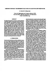
Figure 2: Land data: original, compressed by the factor of 10, and the difference between them
10
Distortion vs. compression ratio 0 -10
Error in Db
-20 -30 -40 -50 -60 Legend Residual amplitude (relative to the original input) Residual amplitude after stack (relative to the original input )
-70 -80 0
10
20
30
40
50
60
70
80
90
100
Compression ratio
Figure 3: Stacking reduces distortion introduced by the transform coding (LCT in this example). [3] A. Cohen, I. Daubechies, and P. Vial. Wavelets on the interval and fast wavelet transforms. Applied and Computational Harmonic Analysis, 1(1):54–81, 1993. [4] I. Daubechies. Orthonormal bases of compactly supported wavelets. Comm. Pure and Appl. Math., 41:909–996, 1988. [5] I. Daubechies. Ten Lectures on Wavelets. CBMS-NSF Series in Applied Mathematics. SIAM, 1992. [6] A. Haar. Zur Theorie der orthogonalen Funktionensysteme. Mathematische Annalen, pages 331–371, 1910. [7] D. Huffman. A method for the construction of minimum redundancy codes. Proc. of IRE, 40:1098–1101, 1952. [8] S. Mallat. Review of multifrequency channel decomposition of images and wavelet models. Technical Report 412, Courant Institute of Mathematical Sciences, New York University, 1988. [9] S. Mallat. A Wavelet Tour of Signal Processing. Academic Press, San Diego, 1998. [10] Y. Meyer. Wavelets and operators. In N.T. Peck E. Berkson and J. Uhl, editors, Analysis at Urbana. London Math. Society, Lecture Notes Series 137, 1989. v.1.
11
[11] R. Ergas P. Donoho and J.D. Villasenor. High-performance seismic trace compression. Soc. Expl. Geophys, 1995. 65th Annual Intern. Conv. Soc. Expl. Geophys. [12] E.C. Reiter and P.N. Heller. Wavelet transformation-based compression of nmo-corrected cdp gathers. Soc. Expl. Geophys, 1994. 64th Annual Intern. Conv. Soc. Expl. Geophys. [13] J.M. Shapiro. Embedded image coding using zerotrees of wavelet coefficients. IEEE Trans. Signal Processing, 41(12):3445–3462, 1993. [14] M. J. Smith and T. P. Barnwell. Exact reconstruction techniques for tree-structured subband coders. IEEE Transactions on ASSP, 34:434–441, 1986. [15] A.A. Vassiliou and M.V. Wickerhauser. Comparison of wavelet image coding schemes for seismic data compression. Soc. Expl. Geophys, 1997. 67th Annual Intern. Conv. Soc. Expl. Geophys. [16] I. Witten, R.Neal, and J. Cleary. Arithmetic coding for data compression. Comm. of the ACM, 30(6):519–540, 1987.
12