Mixed Driver Intention Estimation and Path Prediction Using Vehicle

Mixed Driver Intention Estimation and Path Prediction Using Vehicle Motion and Road Structure Information Master’s thesis in Systems, Control & Mechatronics

Ivar Salomonson, Karthik Murali Madhavan Rathai

Department of Signals and Systems C HALMERS U NIVERSITY OF T ECHNOLOGY Gothenburg, Sweden 2015

Master’s thesis 2015

Mixed Driver Intention Estimation and Path Prediction Using Vehicle Motion and Road Structure Information Ivar Salomonson, Karthik Murali Madhavan Rathai

Department of Signals and Systems Chalmers University of Technology Gothenburg, Sweden 2015

Mixed Driver Intention Estimation and Path Prediction Using Vehicle Motion and Road Structure Information Ivar Salomonson, Karthik Murali Madhavan Rathai

© Ivar Salomonson, Karthik Murali Madhavan Rathai, 2015.

Supervisor: Andrew Backhouse, Volvo Car Corporation Examiner: Lennart Svensson, Department of Signals and Systems

Master’s Thesis 2015 Department of Signals and Systems Chalmers University of Technology

Cover: Path predictions during a lane change maneuver. Typeset in LATEX Gothenburg, Sweden 2015 iv

Mixed Driver Intention Estimation and Path Prediction Using Vehicle Motion and Road Structure Information Ivar Salomonson, Karthik Murali Madhavan Rathai Department of Signals and Systems Chalmers University of Technology

Abstract The development within active safety and driver assistance systems is important in order to reduce the number of traffic related deaths and injuries. For example, collisions can be avoided through automatic steering or braking of the vehicle. The driver can also be alerted about possible threats, e.g. via alarm systems or displays. An important challenge within active safety is to correctly asses a situation in order to intervene only when necessary. For instance, if the system frequently alerts the driver in situations when it is not necessary, then the driver might turn it off. Some active safety systems, such as collision mitigation by braking, use predicted paths of other vehicles for assessing threats. Therefore, improving the accuracy of the path predictions for other vehicles would improve the threat assessment for these systems. One way of improving the path predictions is to consider how the vehicle moves in relation to its surroundings. This thesis proposes an algorithm to predict the paths of traffic participants, that takes the driver intention and road geometry into account. The driver intention is estimated using support vector machines. The predicted path is then generated by combining a motion model prediction and a long term prediction in which the final lateral road placement depends on the driver intention. The algorithm has been tested on object data and the results show that including the driver intention can improve the path prediction in lane change scenarios, but that there are still several challenges to overcome. These challenges include the quality of the road structure information, handling misclassifications and tuning of several parameters.

Keywords: Driver intention, Path prediction, Road structure information, Motion models, Support vector machine. v

Acknowledgements We would like to express our gratitude to our supervisor Andrew Backhouse at VCC and examiner Lennart Svensson at Chalmers University of Technology, for providing their support, guidance and channelizing our potential in the right direction during the pursuit of this thesis.

Ivar Salomonson and Karthik Murali Madhavan Rathai, Gothenburg, October 2015

vii

List of Figures 1.1

1.3

The blue vehicle is oncoming with a large yaw rate. This might cause a false warning since the predicted trajectories intersect. . . . . . . . Two scenarios in which the inclusion of road structure information can change the threat assessment. Note that the vehicles drive on the left side of the road. . . . . . . . . . . . . . . . . . . . . . . . . . An illustration of the overall hierarchy of the proposed approach . . .

2.1 2.2 2.3 2.4

The separating hyperplane can be created in several different ways . Transitions between some rectilinear and curvilinear motion models Object moving in a 2D curve . . . . . . . . . . . . . . . . . . . . . . Infinitesimal travel distance ds of object in time dt . . . . . . . . .

1.2

3.1 3.2 3.3 3.4 3.5 3.6

Lateral position feature of the object with respect to the lane center Constructed grid space in each lane on the road . . . . . . . . . . . Trajectories from the initial to the final states . . . . . . . . . . . . Example of a sequence of the features for a right lane change. . . . Example of a sequence of the features for a left lane change. . . . . Selection of the optimal trajectory from a set of constructed trajectories for a left lane change . . . . . . . . . . . . . . . . . . . . . . . 3.7 Optimization function to determine the optimal time for lane change at a given instance . . . . . . . . . . . . . . . . . . . . . . . . . . . 3.8 Transformation of the trajectory from N-T coordinates to Cartesian coordinates . . . . . . . . . . . . . . . . . . . . . . . . . . . . . . . 3.9 An object’s position is measured from the host vehicle. . . . . . . . 3.10 The host vehicle has moved and hence, the object’s position is measured in another coordinate system. . . . . . . . . . . . . . . . . . . 4.1 4.3 4.4 4.5 4.6 4.7 4.8

3

3 6

. 9 . 14 . 17 . 18 . . . . .

22 23 26 27 27

. 32 . 33 . 34 . 36 . 36

Cumulative error distributions. . . . . . . . . . . . . . . . . . . . . . A left lane change seen from the camera. . . . . . . . . . . . . . . . . A left lane change . . . . . . . . . . . . . . . . . . . . . . . . . . . . . A right lane change . . . . . . . . . . . . . . . . . . . . . . . . . . . . A case where the object is not behaving according to the ground truth An object makes a lane change and is then overtaken by the host vehicle An object makes a lane change and is then overtaken by the host vehicle

40 41 42 43 44 44 45

ix

List of Figures

x

List of Tables 4.1 4.2 4.3

Contingency table for similarity features. P is the predicted intention and GT stands for ground truth, or the actual intention. . . . . . . . 37 Contingency table for lateral position features. P is the predicted intention and GT stands for ground truth, or the actual intention. . . 38 Contingency table for lateral position and similarity features. P is the predicted intention and GT stands for ground truth, or the actual intention. . . . . . . . . . . . . . . . . . . . . . . . . . . . . . . . . . 38

xi

List of Tables

xii

1 Introduction 1.1

Background

Road accidents around the world annually claim the lives of 1.24 million people and injure 20-50 million people. Five pillars are considered to address this; road safety management, safer infrastructure, increased vehicle safety, safer road users and post-crash care [1]. Further, increased vehicle safety plays a significant role in order to reduce the overall number of deaths on European roads [2]. Thus, improved vehicle safety can help decreasing the number traffic related deaths and injuries, in Europe as well as globally. Vehicle safety systems are broadly classified into active and passive safety systems. The latter deal with post-crash safety, such as airbags and seat belts, that mitigate the consequences of a collision while the former deal with pre-crash safety, such as collision avoidance systems and yaw/roll stability systems, which mitigate accidents by predicting safety critical situations and intervene before a situation results in an accident. The key ingredients of an active safety system are sensors, algorithms and system response; the latter consists of either human-machine interface (HMI) or automatic intervention. The sensors monitor the activity around the vehicle and provide data to the processing unit. The algorithms deployed in the processing unit process the sensor data and assess the risk of collision or other safety related issues. The system responds either through the HMI, by providing information/warnings that help the driver assess the situation, or via automatic actuation, such as steering/braking control [16]. One of the most important functions of an active safety system is the collision avoidance system (CAS). The CAS considers three measures to obviate an imminent collision; warning, braking and steering systems. Warning systems alert/warn the driver about a possible collision via visual/auditory stimuli, such as heads up displays or alarm modules, that help the driver take appropriate measures to avert the collision. Braking and steering systems can override the manual control of the vehicle in scenarios when the safety system detects an imminent collision or the vehicle drifts away from the intended lane. Despite its potential functionality, there are certain conditions and constraints about the performance of a CAS. For instance, the braking system has restrictive constraints on the number of false interventions which it should allow, and must intervene only when the situation lands up in an imminent collision. Allowing too many false warnings makes the driver more likely 1

1. Introduction

to disconnect the safety system. The decision making for whether or not the CAS should intervene is done in the threat assessment (TA) module. An important component of the TA module is the collision mitigation by braking (CMbB) system. In [7], the CMbB functionality is triggered only when the the road user cannot avoid a collision neither by applying moderate steering nor by braking. However, waiting until the other road user cannot perform a collision avoidance maneuver leads to that the CAS intervenes late, which increases the risk of collision. Further, in [7], information about the road is excluded in the treat assessment. The importance of including road structure information in in the TA module can be understood from studying some special cases. Fig. 1.1 shows an oncoming vehicle that has a significant yaw rate. Since the predicted paths intersect, the TA module in [7] would probably predict a collision. However, if the situation in Fig. 1.1 is viewed in the context of Fig. 1.2a, then it is probable that the blue vehicle has a high yaw rate because it is following the curved road. Further, the red vehicle is likely to stop or slow down until the blue vehicle has passed. If this is the case, then the situation would not be considered as a threat. If the same situation is viewed in the context of Fig. 1.2b, then the blue vehicle would be coming around the corner with a large yaw rate. Considering the shape of the road, it is plausible that the vehicle’s yaw rate is high because it is following the road. If the blue vehicle follows the road, then the vehicles’ paths do not intersect. Hence, this scenario is not considered as a threat. In summary, including road structure information allows estimating a driver’s intention. Further, the driver intention provides vital information when it comes to predicting the future trajectory of a vehicle. Therefore, path predictions based on road structure information and driver intention can improve the TA module’s decision basis compared to predictions based on the method proposed in [7].

1.2

Problem Formulation

The problem is to develop an algorithm that predicts the future trajectory of road users based on object data, road structure information and the intention of the driver. Road structure data and estimated intentions of drivers will be used to improve the accuracy of the predicted paths. The algorithm should also be scalable such that it could be utilized for several scenarios such as roundabouts, intersections etc.

1.3

Previous Work

There have been several research studies for prediction of vehicle trajectories. According to [26], path prediction can be broadly classified into three levels; physics based, maneuver based and interaction aware motion models. Out of these, the first two will be discussed in this thesis. Physics based motion models predict trajectories by propagating the initial vehicle state over time, using a predefined model. Physics based motion models are further 2

1. Introduction

Figure 1.1: The blue vehicle is oncoming with a large yaw rate. This might cause a false warning since the predicted trajectories intersect.

(a)

Situation 1

(b)

Situation 2

Figure 1.2: Two scenarios in which the inclusion of road structure information can change the threat assessment. Note that the vehicles drive on the left side of the road.

classified into dynamic and kinematic motion models. Dynamic motion models utilize internal parameters of the vehicle that affect its motion, such as forces acting on chassis or wheels, cornering forces etc. [26]. Several dynamic motion models can be found in the works [11], [27], [23], [32]. Kinematic motion models utilize parameters of motion, e.g. velocity and acceleration, but exclude forces acting on the vehicle. Common kinematic motion models include constant velocity, constant acceleration, constant yaw rate and acceleration. A comparative study between different models is performed in [36] and several variants of kinematic motion models are found in 3

1. Introduction

the works [33], [29], [22], [3]. There are several methods to estimate a trajectory using motion models. According to [26], the trajectory could be a single trajectory based on motion models, with or without uncertainty associated to it. Uncertainty can be modeled using Gaussian distributions with methods such as Kalman filters. Research work related to this method are found in the [20], [37], [24], [19]. Maneuver based motion models rely on the maneuver which the driver performs or intends to perform. A maneuver is defined as a physical motion executed by the driver with skill and care. Maneuver based motion models can be composed into prototype trajectories, maneuver intention estimation and maneuver execution [26]. Prototype trajectory methods are based on motion patterns executed by different drivers given the road topology. These patterns are then clustered and used to predict the future trajectory of the vehicle. This task is accomplished by comparing the past trajectory of a vehicle with the motion patterns. There are several metrics to measure the similarity such as average Euclidean distance [34],[40], longest common sub sequence [13], quaternion rotation invariant longest common sub sequence [8]. Intention estimation methods are used to predict what the driver intends to do such as take a left turn, right turn, change lane etc. These methods utilize several parameters such as road structure information or vehicle states and are predominantly predicted using machine learning techniques. Some machine learning methods that have been used for driver intention estimation are hidden Markov models [18], [38], support vector machines [25], [4], [17], and relevance vector machines [4]. From the determined intention, different probabilistic approaches for predicting the trajectories are proposed in the works [9], [10]. In [21], the maneuver intention is estimated using statistical methods. Based upon the intention, the vehicle’s trajectory is then predicted using polynomials in time.

1.4

Datasets

The measurements used in this thesis are provided by Volvo Cars. They are collected with an average sampling time of 0.025 s., using gyro and accelerometer as well as a forward looking camera and radar with detection ranges of 70 and 150 meters respectively. The data are then preprocessed to provide information, such as position, velocity, acceleration, yaw rate and heading angle, about the host vehicle and surrounding objects. Further information in the data sets is road structure information containing lane width, lane marker estimates and the region of validity of the estimates. Moreover, information about host vehicle lane changes is available as the time instance and direction of the lane change. All measurements are represented in a moving coordinate system with origin in the center of the host vehicle’s rear axis and coordinate axes in its forward and lateral directions. The data used in the thesis are collected from two drivers during a three days long drive between Paris and Barcelona. 4

1. Introduction

1.5

Thesis Organization/Proposed Approach

The proposed approach is inspired from [21] which comprises of two stages; estimation of driver intention and prediction of vehicle trajectory. In this thesis, the driver intention is estimated using a support vector machine. The trajectory is predicted by fusing a short term and a long term prediction. The former is predicted using motion models while the latter is predicted using road structure information and the estimated driver intention. The two predictions are then combined to obtain the final prediction. The overall hierarchy of the approach is illustrated in Fig. 1.3.

1.6

Limitations

Several limitations are made due to the content of the used log data as well as to limit the complexity of the work. First, as mentioned the log data contains information about host vehicle lane changes. However, there is no corresponding information about for other vehicles. Therefore, host vehicle data is used for training the support vector machine. Second, the log data contains no additional information, beyond the lane change information, that can be used for labelling. Therefore, the intentions are limited to keep lane, left lane change and right lane change. However, it is emphasized that the features should be useful also in case of a future extension of the number of classes. Third, only consider cars and trucks are considered in the evaluation of the algorithm. Fourth, inter vehicular dependencies are not considered. Finally, only a subset of the log data are used, due to that the quality of the road geometry information in the log data varies. A description of the log data selection is provided in chapter 3.

5

1. Introduction

Figure 1.3: An illustration of the overall hierarchy of the proposed approach

6

2 Theoretical Framework This chapter gives an overview of the theory used in this thesis. First, some basic machine learning concepts are introduced. Second, the support vector machine is derived. Third, some methods to extend the SVM to multiclass problems are discussed. Fourth, some motion models are introduced and finally, the basics about road coordinate systems are presented.

2.1

Machine Learning

The goal of machine learning is to make conclusions about new data based on previous knowledge [15]. Machine learning problems are broadly classified into three categories; supervised, unsupervised, and reinforced learning [6]. In machine learning, the input data are represented by vectors X = (x1 , x2 , ...xn ). These are often termed feature vectors, input vectors, samples, examples, or pattern vectors. The components of feature vectors are often called features, attributes, components or input variables, and can contain discrete or real valued numbers. In supervised learning, the input vectors are each associated with an output value, which is typically called class, decision, category or label. The learning algorithm, which is often called classifier, categorizer or recognizer then tries to fit the examples to the labels. Another way of mapping attributes to categories is unsupervised learning. In contrast to supervised learning, unsupervised learning algorithms find patterns in the data without given labels [31]. The third category is known as reinforcement learning. The goal of reinforcement learning is to find actions that maximise the reward in a given situation [6].

2.1.1

Cross Validation

When training a classifier there are often several parameters to tune. The optimal parameters are the ones that give the best classification accuracy on new data. A common way to estimate this accuracy is to use k-fold cross-validation. In k-fold cross-validation, the data is split into k groups. Then k-1 groups are used for training the classifier and the last group is used for validation. The estimated performance is then the mean value of the k tests. Usually, k is set to 5 or 10 [39]. 7

2. Theoretical Framework

2.2

Support Vector Machines

A support vector machine (SVM) is a classifier for supervised learning. When training SVMs, a hyperplane that separates the input data in accordance with their labels is created. New feature vectors are then classified according to which side of the hyperplane they belong to. The usefulness of support vector machines is greatly enhanced by the possibility to employ kernel functions. They provide a tool for efficiently mapping the input vectors to a higher dimensional space where nonlinear feature dependencies can be evaluated. The support vector machine will be derived in two steps based on lecture notes from Andrew Ng [30]. First, an optimization problem for linear maximum margin separation of data will be derived. Second, the problem is reformulated the allow the utilization of kernel functions. The two problems are denoted as the primal and the dual problem.

2.2.1

The Primal Optimization Problem

The equation of a hyperplane is ωT x + b = 0

(2.1)

where ω is a vector that is orthogonal to the hyperplane and b is the bias of the hyperplane. Any sample x for which this equation is satisfied, describes a point on the hyperplane. For samples not on the hyperplane, the output of Eq. (2.1) has either positive or negative sign depending on which side of the hyperplane the sample is. The classifier relies on this and is expressed as h(x) = g(ω T x + b) = g(z) where g(z) =

 1,

if z ≥ 0 −1, otherwise

(2.2)

(2.3)

As can be seen in Fig. 2.1, two sets of feature vectors can be separated in different ways and therefore a method to decide the optimal separating hyperplane is needed. This is achieved by finding parameters ω and b, such that the minimum Euclidean distance between the hyperplane and any point in the training set is maximized. This distance is called the geometric margin and is denoted γ. An expression for the geometric margin can be obtained as follows: Consider an input vector xi (y i is disregarded for now) and its projection p on the hyperplane. Since ω/kωk is a unit vector normal to the hyperplane, then p can be found as ω p = x(i) − γ (i) kωk

(2.4)

Since p is on the hyperplane, it can be inserted in in Eq. (2.1). This yields !

ω

T

x

(i)

ω −γ +b=0 kωk

Solving for the geometric margin gives 8

(i)

(2.5)


Class 1 Class -1 Support Vectors Decision Boundary

x2

x2

Class 1 Class -1 Decision Boundary

x1

x1

A decision boundary with maximum margin

Some possible decision boundaries with non-maximum margin

(a)

(b)

Figure 2.1: The separating hyperplane can be created in several different ways

γ

(i)

ω = kωk

!T

x(i) +

b kωk

(2.6)

More generally, i.e. considering that x(i) can be located on both sides of the hyperplane, the geometric margin can be written as 

γ (i) = y (i) 

ω kωk



!T

x(i) +

b  kωk

(2.7)

The idea now is to find the hyperplane that separates pattern vectors according to their label, and at the same time maximizes the geometric margin. This can be set up into the following optimisation problem max γ γ,ω,b

s.t. y (i) (ω T x(i) + b) ≥ γ kωk = 1

(2.8)

Even though solving this optimisation problem would give the optimal hyperplane, the constraint on ω makes the problem non convex. This can be solved by instead maximizing γˆ /kωk while constraining γˆ to be equal to 1. Since maximizing γˆ /kωk is equivalent to minimizing kωk, then a new optimization problem, still giving the optimal hyperplane, can be set up as min 12 kωk2 s.t. y (i) (ω T x(i) + b) ≥ 1

(2.9)

where the factor 1/2 is included for mathematical convenience. This gives a convex optimization problem which can be solved efficiently. The above problem is called the primal optimization problem. It can be transformed into a dual problem by using Lagrange multipliers. For the dual problem, it 9


is possible to write the solution in terms of dot products between the feature vectors, which in turn allows the utilization of kernel functions.

2.2.2

The Dual Optimization Problem

Since the derivation of the dual optimization problem relies on the usage of Lagrange multipliers, this section starts with providing a brief description of Lagrange multipliers and how they connect the primal and the dual optimization problems. After that follows the derivation of the dual optimization problem. An optimization problem that has the form min f (x) s.t. gi (x) ≤ 0, i ∈ {1, ..., m} s.t. hi (x) = 0, i ∈ {1, ..., n}

(2.10)

where g and h represent equality and inequality constraints respectively can, using Lagrange multipliers, be rewritten as max f (x) +

m P

αi gi (ω) +

n P

βi hi (ω)

i=1

i=1

s.t. gi (x) ≤ 0, i ∈ {1, ..., m} hi (x) = 0, i ∈ {1, ..., n} αi ≥ 0, i ∈ {1, ..., m}

(2.11)

where α and β are Lagrange multipliers and the objective function is called the Lagrangian or L. If the constraints are fulfilled, then the solution to this problem will be the same as the solution to the original problem. Thus, with the same constraints, the primal problem can be written as min max ω

α,β:αi ≥0

L(ω, b, α)

(2.12)

The dual problem is then obtained by altering the order of the minimization and maximization and hence has the form max min L(ω, b, α)

α,β:αi ≥0

ω

(2.13)

The solution of the dual problem will always be smaller or equal to the solution of the primal problem. The two problems have identical solutions if the KKT conditions are fulfilled. They are as follows: ∂ L(ω ∗ , α∗ , β ∗ ) = 0, i = 1, ..., n ∂ωi ∂ L(ω ∗ , α∗ , β ∗ ) = 0, i = 1, ..., l ∂βi αi∗ gi (ω ∗ ) = 0, i = 1, ..., k gi (ω ∗ ) ≤ 0, i = 1, ..., k α∗ ≥ 0, i = 1, ..., k 10

(2.14) (2.15) (2.16) (2.17) (2.18)

2. Theoretical Framework where ω ∗ is the optimal solution to the primal problem and α∗ , β ∗ provide the optimal solution to the dual problem. Employing this on the optimization problem for support vector machines, the Lagrangian can be written according to m X 1 2 L(ω, b, α) = kωk − αi [y (i) (ω T x(i) + b) − 1] 2 i=1

(2.19)

In order write the problem in its dual form, L(ω, b, α) is differentiated w.r.t. ω and b according to m X ∂L(ω, b, α) =ω− αi y (i) x(i) = 0 ∂ω i=1

⇒ω=

m X

αi y (i) x(i)

(2.20)

(2.21)

i=1 m ∂L(ω, b, α) X αi y (i) = 0 = ∂b i=1

(2.22)

By inserting Eq. (2.21) into Eq. (2.19) and simplifying, the following expression is obtained m m m X X 1X (i) (i) (j) (i) T (j) αi − αi αj y y (x ) x − b αi L(ω, b, α) = 2 i=1 j=1 i=1 i=1 m X

(2.23)

Since Eq. (2.22) states that the last term must be zero the dual optimization problem can be written as m P

max α

αi −

i=1 Pm i=1

s.t.

1 2

m P m P

y (i) y (j) αi αj (x(i) )T x(j)

i=1 j=1

αi y (i) = 0, i ∈ {1, ..., m} αi ≥ 0, i ∈ {1, ..., n}

(2.24)

Once the dual optimization problem is solved, ω can be obtained from Eq. (2.21). The bias b can then be calculated from the support vectors as b=

−maxi:y(i) =−1 ω ∗T x(i) + mini:y(i) =1 ω ∗T x(i) 2

(2.25)

New data can then be evaluated according to ωT x + b =

 T m X  αi y (i) x( i) i=1

x+b=

m X

αi y (i) (x(i) )T x + b

(2.26)

i=1

This shows that only the support vectors are needed to evaluate new data. This can also be seen in Fig. 2.1a. Furthermore, the dot product can be replaced with a kernel function. The benefit of that will be shown in the next section. 11


2.2.3

Kernel Functions

Kernel functions can be used whenever there is a dot product between two vectors x and z. Instead of directly evaluating the dot product, the kernel function evaluates the dot product between φ(x) and φ(z), which are functions mapping the original vectors to a higher dimensional space. As an example the kernel function K(x, z) = (xT z)2 can be considered. In the case of two dimensional vectors this yields K (x, z) = (x1 z1 + x2 z2 )2 = x21 x22 + 2x1 z1 x2 z2 + x22 z22

(2.27)

Expressed in terms of the vector mappings this becomes 



2  √ z1 √  2 2  T x1 , 2x1 x2 , x2  2z1 z2   = φ(x) φ(z) z22

(2.28)

For higher vector dimensions the corresponding calculation becomes 2

K(x, z) = (x1 z1 , ..., xn zn ) =

   n n X X  xi zi   xj zj  i=1

j=1

=

n X n X

xi xj zi zj

(2.29)

i=1 j=1

where n is the vector dimension. In this case the mapping of the feature vector x becomes φ(x) = (x1 x1 ...x1 xn ...xn x1 ...xn xn )T (2.30) This means that calculating the mapped feature vectors has the complexity O(n2 ), while evaluating the kernel function only has the complexity O(n). As seen above, calculating the mappings can be costly for high vector dimensionality. However, the kernel function can be evaluated without calculating φ(x) and φ(z). This gives the advantage of the high dimensionality, i.e. to be able to (sometimes) separate feature vectors that are not separable in the original space, without having to pay the full cost in terms of calculational complexity [30].

2.2.4

Common SVM Kernels

Some kernels that are often used in support vector machines are the Linear kernel: xT z Polynomial kernel: (xT z + c)d . Radial basis kernel: e(−γkx−zk) Sigmoid kernel: tanh(xti xj + r) If the data are linearly separable, then the linear kernel is a good choice because 12


the training can be done quickly with good performance. The other kernels can be good choices if the relation between the feature vectors and the classes is nonlinear [12].

2.2.5

Soft Margin SVM

Although employing kernel functions can help separating data that are not linearly separable in the original feature space, separation of all data is sometimes not possible. For example, this can be the case if there are outliers. If the data are not linearly separable even after employing kernel functions, then the SVM formulation as stated in Eq. (2.24) cannot be applied. However, this becomes possible by modifying the SVM formulation to a soft margin SVM. The soft margin SVM is obtained by introducing slack variables and is derived similarly to the original SVM. The resulting problem is formulated as follows: min kωk2 + C s.t. y (i) (ω T x

m P

ξi

i=1 (i)

+ b) ≥ 1 − ξi ξi > 0

(2.31)

where ξ is either the geometric margin of a misclassified feature vector and C is a cost parameter. The dual problem, which is derived similar to before, then has the form max α

s.t.

m P

αi −

i=1 Pm i=1

1 2

m P m P

y (i) y (j) αi αj (x(i) )T x(j)

i=1 j=1 (i)

αi y = 0, i ∈ {1, ..., m} 0 ≤ αi ≤ C, i ∈ {1, ..., n}

(2.32)

The only difference from Eq. (2.24) is that αi must also be smaller or equal to C.

2.2.6

Extension to multiple classes

Although support vector machine were originally created for binary classification problems, several methods have been suggested for treating multiclass problems. Three methods that commonly occur in the literature are one-versus-all, one-versusone and DAG-SVM. In the one-versus-all approach k SVMs are created, which is equally many as the number of classes. Each SVM compares the data from one class to the data from all other classes. A drawback of this method is the possibility that one data vector is associated with several classes. In that case the distance to the hyperplane can be used to make a decision. However, this might be problematic if the the distances to the different hyperplanes do not have the same scale. This might be the case since the classifiers were not trained for the same task. Another problem with the one-versus-rest approach is that the training sets are unbalanced, i.e. there are several more samples of one class. This might cause the decision boundary to be biased toward the class with more examples. A method that is also commonly used is to create k(k − 1)/2 classifiers, each separating two classes. The output from each classifier counts as a vote, and the class 13


Figure 2.2: Transitions between some rectilinear and curvilinear motion models with highest number of votes is chosen. A drawback of this method is the possibility that several classes get equally many votes. Furthermore, the time needed for classification and training is large, compared to other methods, if there are many classes. The DAG-SVM is another multi-SVM approach. It organises k(k − 1)/2 classifiers into a graph such that only k − 1 classifiers need to be evaluated for testing new data [6].

2.3

Motion Models

Motion models are mathematical frameworks, which can be used to predict the future state of a vehicle using the current state [36]. Motion models accurately explain the evolution of the vehicle trajectory for a short time due to the inertia of the vehicle [21]. It is possible to construct different motion models depending upon the set of observed measurements and whether the state update is linear or non linear. Roughly, motion models can be divided into models that consider rotation (curvilinear motion models) and models which do not consider rotation (rectilinear motion models). Two examples of models that belong to the former group are the constant turn rate and velocity (CTRV) and the constant turn rate and acceleration (CTRA) models while two models which belong to the latter group are the constant velocity (CV) and constant acceleration (CA) models. The relation between these models is graphically illustrated in Fig. 2.2. These four models will now be described shortly. 14


2.3.1

Constant Velocity Model

The constant velocity (CV) model is a linear and rectilinear motion model which considers a constant velocity for the motion of the vehicle. The state vector for h iT the CV model is given as X(k) = x vx y vy and the state update equation is given as 



1 ∆T 0 0   0 1 0 0   X(k)  X(k + 1) =  0 1 ∆T   0 0 0 0 1

(2.33)

where x is the longitudinal position of the vehicle, vx is the longitudinal velocity of the vehicle, y is the lateral position of the vehicle, vy is the lateral velocity of the vehicle and ∆T is the sample time.

2.3.2

Constant Acceleration Model

The constant acceleration (CA) model is a linear and rectilinear model, like the constant velocity model, which considers a constant acceleration for the motion of the h iT vehicle. The state vector for the CA model is given as X(k) = x vx ax y vy ay and the state update equation is given as 

1 ∆T ∆T 2 /2  0 1 ∆T  0 0 1  X(k + 1) =  0 0 0  0 0 0  0 0 0



0 0 0  0 0 0   0 0 0    X(k) 2 1 ∆T ∆T /2  0 1 ∆T   0 0 1

(2.34)

where x is the longitudinal position of the vehicle, vx is the longitudinal velocity of the vehicle, ax is the longitudinal acceleration of the vehicle, y is the lateral position of the vehicle, vy is the lateral velocity of the vehicle, ay is the lateral acceleration of the vehicle and ∆T is the sample time.

2.3.3

Constant Turn Rate and Velocity Model

The constant turn rate and velocity (CTRV) model is a nonlinear and curvilinear h

motion model. The state vector for the CTRV model is X(k) = x y θ v ω

iT

15


and the state update equation is given as  v v  ω sin(ω∆T + θ) − ω sin(θ) + x(k)    

X(k + 1) =

   v − cos(ω∆T  ω     



 v  + θ) + sin(θ) + y(k)  ω   ω∆T + θ   v  ω

(2.35)

where x is the longitudinal position of the vehicle, y is the lateral position of the vehicle, θ is the heading angle of the vehicle, v is the velocity of the vehicle, ω is the yaw rate of the vehicle and ∆T is the sample time.

2.3.4

Constant Turn Rate and Acceleration Model

The constant turn rate and acceleration model (CTRA), also known as constant yaw rate and acceleration (CYRA), is a nonlinear and curvilinear motion model which involves linear variation of the curvature [36]. The state vector for the CTRA model h

is X(k) = x y θ v a ω

iT

and the state update equation is given as 







∆x(∆T ) x(k + 1)     ∆y(∆T ) y(k + 1)      ω∆T   θ(k + 1)       = X(k) +   X(k + 1) =   a∆T  v(k + 1)         a 0     0 ω with 1 [(v(k)ω + aω∆T ) sin(θ(k) + ω∆T ) ω2 +a cos(θ(k) + ω∆T ) − v(k)ω sin θ(k) − a cos θ(k)] ∆x(∆T ) =

and 1 [(−v(k)ω − aω∆T ) cos(θ(k) + ω∆T ) ω2 +a sin(θ(k) + ω∆T ) + v(k)ω cos θ(k) − a sin θ(k)]

∆y(∆T ) =

where x is the longitudinal position of the vehicle, y is the lateral position of the vehicle, θ is the heading angle of the vehicle, 16

(2.36)


Figure 2.3: Object moving in a 2D curve v is the velocity of the vehicle, a is the acceleration of the vehicle, ω is the yaw rate of the vehicle and ∆T is the sample time.

2.4

Normal-Tangent Coordinate System

The normal-tangent (N-T) coordinate system is a curvilinear coordinate system, which is used when an object moves along a predefined path or profile [14]. The coordinate system is described by two orthogonal unit vectors; the normal vector ~ and the tangent vector T~ . The origin of the coordinate system always coincides N with the location of the object on the profile. An example of an N-T coordinate system for an object, X, moving along a curve is found in Fig. 2.3. The object has traversed an arc distance s(t) along the profile from the point O. The tangent vector ~ is perpendicular to T~ , T~ is tangential to the curve at X and the normal vector N 0 with direction towards the center of curvature O . In addition, the corresponding coordinate system in three dimensions is known as tangent-normal-binormal (TNB) or Frenet-Serret frame.

2.4.1

Equations of Motion in the N-T Coordinate System

Since the object moves along the profile, the object traverses along a curved distance which is a function of time expressed as s(t). The velocity of the object always remains tangential to the profile and the magnitude of the velocity is given as v = v T~ , where v = s(t) ˙

(2.37) (2.38) 17


Figure 2.4: Infinitesimal travel distance ds of object in time dt The acceleration of the object in the N-T coordinate system is determined by the time derivative of the velocity, which is a = v˙ = v˙ T~ + v T~˙

(2.39)

where T~˙ is the rate of change of the tangent vector along the profile and is determined from the assumption that the object travels an infinitesimal arc length ds in time dt. As the direction of T~ changes over time, the magnitude is unity at all times ! ~ ~0 ~ T = T = 1 T˙ .

~ , where dT ~ = dθN ~ . Taking the From figure 2.4, resolving the vectors T~ 0 = T~ + dT derivative with respect to time, ~ = vN ~ T~˙ = θ˙N r

(2.40)

substituting the normal and tangential components, the acceleration of the object is given as, ~ a = at T~ + an N (2.41) q v2 and the magnitude is given as a = a2n + a2t . If the path is r described as y = f (x), then the radius of curvature is given as

where at = v, ˙ an =

[1 + (dy/dx)2 ]3/2 r= d2 y/dx2

2.4.2

Special Cases

There are two important cases of motion in an N-T coordinate system [14]. 18

(2.42)


1. If the object moves on a linear profile, then the curvature is zero. This means that the radius r → ∞ and therefore an = 0. Therefore, only the tangential component of the acceleration exists, which is at = v. ˙ 2. If the object moves on a curved profile with constant speed, then the tangential component of acceleration is at = v˙ = 0 and the normal component of v2 acceleration is an = r

19


20

3 Implementation This chapter describes the implementation aspects of the work. First, it is described how the features are calculated. Second, an overview of how the feature vectors are extracted from the log data and labelled is provided. Third, a detailed explanation of the proposed path prediction is given and finally, it is explained how the predicted paths are evaluated.

3.1

Features

As described in the theory chapter, any real valued or discrete number can be used as a feature. However, it is important to choose features that are correlated with the actual intention in order for the support vector machine to make accurate classifications. Some examples of possible features in lane change classification are vehicle states, such as velocity and acceleration, road structure data, like road curvature and lane marker estimates, or combinations of several measurements. From [35], it is evident that the lateral position, lateral velocity and the longitudinal velocity relative to the preceding vehicles possess the maximum predictive power. Also in [25], [28], a similar feature space is utilised as input to the SVM. In this thesis, the features include the lateral position with respect to the lane center, as well as a new feature called similarity feature. The choice of features was made such that the features should not only be correlated with lane change intentions, but also be applicable to an extended number of classes. The chosen features are described below.

3.1.1

Lateral Position

The lateral position is equal to the signed Euclidean distance between the object and the lane center as displayed in Fig. 3.1. It is calculated as follows: The object’s position with respect to the host vehicle is given as (xobj , yobj ) and the lane center is described by a third order polynomial according to f (x) = a3 x3 + a2 x2 + a1 x + a0

(3.1)

If (x, y) represents any position on the lane center, then the squared distance between the object and the lane center curve can be expressed as D2 = (x − xobj )2 + (y − yobj )2

(3.2)

Substituting f (x) in the above equation yields 21

3. Implementation

Figure 3.1: Lateral position feature of the object with respect to the lane center

D 2 = b6 x 6 + b5 x 5 + b4 x 4 + b3 x 3 + b2 x 2 + b1 x + b0

(3.3)

where the coefficients bi|i=0...6 are given as     b6      b5        b4 

b

3     b2       b1       b0

= a23 = 2a2 a3 = 2a1 a3 + a22 = 2a1 a3 + 2a1 a3 − 2a3 yobj = a21 + 2a0 a2 − 2a2 yobj + 1 = 2a0 a1 − 2a1 yobj − 2xobj 2 = a20 − 2a0 yobj + x2obj + yobj

(3.4)

From minimizing the squared distance (D2 ), the x-coordinate of the object’s projection on the lane center is obtained as xroad = min D2 x

(3.5)

The y-coordinate of the projection can then be obtained from Eq. (3.1) according to yroad = f (xroad ) (3.6) Next, the shortest distance between the object and the lane center is computed as q

D = ± (xroad − xobj )2 + (yroad − yobj )2

(3.7)

In order to determine on which side of the lane center the object is, D is considered to be negative if the object is to the right of the lane center. 22

3. Implementation

Figure 3.2: Constructed grid space in each lane on the road

3.1.2

Similarity Feature

The similarity feature is a novel feature introduced in this thesis. It describes the similarity between a motion model prediction and multiple hypothesis paths connecting the object’s current state with possible future states. As stated in section 2.3, motion model predictions accurately describe the motion of a vehicle during a short time due to the inertia of the vehicle. There are several measures to determine the similarity between two trajectories [42]. In this thesis the root mean square (RMS) error is utilized. A more detailed description of how the feature is calculated follows below. The initial state vector of the object is given as h

Xinit = x0 y0 θ0 v0 a0 ω0

iT

(3.8)

The distance that the object will have travelled in a near future, assuming constant acceleration, is calculated using the kinematic equation 1 (3.9) Stravel = v0 ttravel + a0 t2travel 2 In the implementation ttravel is assumed to be 2 s. The future coordinates of the object are determined based on the assumptions xroad = x0 + Stravel yroad = f (xroad )

(3.10) (3.11) 23

3. Implementation

where f is expressed in Eq. (3.1). The point (xroad , yroad ) constitutes a basis to generate the grid space, which is a set of equally spaced points on the road that describe the final positions of the hypothesis paths. The grid space is described for each of the classes; in this case the lanes of the road are considered. The grid length, (GL ), is the number of grid points along the longitudinal axis and the grid breadth, (GB ), is the number of grid points along the lateral axis. The grid dimension for each lane is given by the product between (GL ) and (GB ). The horizontal spacing ∆x between the grid points is assumed to be constant. In the implementation, ∆x is assumed to be 5 m and (GL ) as well as (GB ) are set as 3. Further, the vertical spacing is constrained to be within the boundaries of the lane width of the individual lanes. An example of the grid space implementation is seen in Fig. 3.2. So far, the final positions of the grid space have been determined. However, in order to construct the hypothesis path trajectories, the initial and final states are required. The initial vehicle state is given is Eq. (3.8) and the derivation of the final states follows. The fundamental assumptions to deduce the final state vector is that the object follows the road profile and maintains the same acceleration. From these assumptions, the end state vector for each grid point is computed as shown below. Let the classes be represented by C ∈ {Lef t, Right, Center}, i represent the index of the grid length and j represent the index of the grid breadth. The coordinates of grid point (i, j) for the C th class is denoted as (xC (i, j), yC (i, j)). Each variable of the final state vector will now be calculated separately. The assumption that the object follows the road implies that the object’s final heading angle is the same as the road tangent at that position. This is expressed as θC (i, j) =

  π

0

− tan−1 f (x)|xC (i,j) , if the vehicle is oncoming

 tan−1

0

f (x)|xC (i,j) ,

otherwise

(3.12)

The distance from the object’s initial position to its final position is given as DC (i, j) =

q

(xC (i, j) − x0 )2 + (yC (i, j) − y0 )2

(3.13)

The final velocity is then determined according to q

vC (i, j) = ± v02 + 2a0 DC (i, j)

(3.14)

The final yaw-rate of the object is determined from the equation ωC (i, j) =

(afy in vxf in − afxin vyf in ) (vxf in )2 + (vyf in )2

where vxf in = v0 cos(θC (i, j)) is the final velocity along the longitudinal axis, vyf in = v0 sin(θC (i, j)) is the final velocity along the lateral axis, afxin = a0 cos(θC (i, j)) is the final acceleration along the longitudinal axis and afy in = a0 sin(θC (i, j)) is the final acceleration along the lateral axis. 24

(3.15)

3. Implementation

Thus, the final state vector is given as 



x (i, j)   C  yC (i, j)     θ (i, j)    C C  Xf in (i, j) =   vC (i, j)     a (i, j)    C ωC (i, j)

(3.16)

When both the initial and final state vectors are calculated, the consecutive step is to generate trajectories that connect them. The longitudinal and lateral trajectories are each modeled as a quintic time polynomial; this gives a unique solution and a jerk continuous trajectory [41], [21]. The longitudinal trajectory and its derivatives are given as     

x(t) = cx0 + cx1 t + cx2 t2 + cx3 t3 + cx4 t4 + cx5 t5 x(t) ˙ = cx1 + 2cx2 t + 3cx3 t2 + 4cx4 t3 + 5cx5 t4     x ¨(t) = 2cx2 + 6cx3 t + 12cx4 t2 + 20cx5 t3

(3.17)

The lateral trajectory and its derivatives are given as     

y(t) = cy0 + cy1 t + cy2 t2 + cy3 t3 + cy4 t4 + cy5 t5 y(t) ˙ = cy1 + 2cy2 t + 3cy3 t2 + 4cy4 t3 + 5cy5 t4     y¨(t) = 2cy + 6cy t + 12cy t2 + 20cy t3 5 4 3 2

(3.18)

The trajectory is modeled with polynomials in time and the time for the object to reach the final state is computed from the relation

TC (i, j) =

   |vC (i, j)| + |v0 |   ,   a0  

if a0 6= 0

     DC (i, j)  ,   v0

if a0 = 0

(3.19)

Next, the polynomial coefficients need to be determined. In order to determine the polynomial coefficients, the initial and final state vectors are transformed to lateral and longitudinal position, velocity and acceleration according to 



 

x y  s    ys  y˙      θ  y¨  s     7−→    vs  x     a  x˙   s   ωs x¨

(3.20)

25

3. Implementation

Figure 3.3: Trajectories from the initial to the final states where the transformation relation is given as   y = ys       y˙ = vs sin(θs )      y¨ = as sin(θs ) + vs ωs cos(θs )  x       x˙     x ¨

(3.21)

= xs = vs cos(θs ) = as cos(θs ) − vs ωs sin(θs )

By substituting the initial and final conditions, the coefficients of the polynomial are calculated and the longitudinal and lateral trajectories are determined. An example of multiple hypothesis trajectories generated in this way is seen in Fig. 3.3. As mentioned, the similarity between the hypothesis paths and a motion model prediction of the vehicle’s path is calculated using the RMS error. In this thesis the CA-model is used for predicting the vehicle’s motion for a time period Ts = 1 s. If the length of the CA prediction is M and the length of the generated trajectory N , then the similarity measure is computed according to

dC (i, j) =

v u u X t CA

− XTCraj (i, j)

T

XCA − XTCraj (i, j)

(3.22) L where L = min{M, N } and the trajectories are represented as XCA = {(x1 , y1 ), (x2 , y2 )...(xM , yM )} and XTCraj (i, j) = {(x1 , y1 ), (x2 , y2 )...(xN , yN )}. For each considered lane, the similarity that best fits the vehicle motion is selected as

(3.23)

P

SimC = 1. This ensures

SimC = min min dC (i, j) i∈GL j∈GB

The similarity feature is then normalized such that that the feature is scaled between 0 and 1. 26

C

3. Implementation

1

Feature value

0.5 0 -0.5 -1 Sim right Sim left Sim center Lateral position

-1.5 -2 0

100

200

300 Sample

400

500

Figure 3.4: Example of a sequence of the features for a right lane change.

2 1.5

Feature value

1 0.5 0 -0.5 Sim right Sim left Sim center Lateral position

-1 -1.5 0

500

1000

1500

Sample

Figure 3.5: Example of a sequence of the features for a left lane change.

3.2

Training the Support Vector Machine

In order to be able to train the SVM, the features have to be organized as feature vectors and furthermore, each feature vector needs a label. How that was done is described in this section. 27

3. Implementation

3.2.1

Data Selection

The possibility to calculate the features depends on the data. In order to calculate the lateral position feature, the lane width is needed. Further, when calculating the similarity features, the ability to place the grid points correctly depends on the accuracy of the lane marker estimates. However, the log data does not always contain lane marker estimates. Moreover, even if lane marker estimates do exist, their accuracy is most of the time not sufficient for calculating the similarity features. Another factor that was considered in the data selection is that the considered objects should be moving. In order to find suitable data, the log files were searched for data fulfilling certain constraints. First, the lane marker estimates should be accurate enough until the longitudinal position reached 2 seconds into the future, assuming constant acceleration. This was decided using predefined accuracy measures in the log data. Even though the final position is often placed further away than that, it was found that a higher threshold did not leave much data to analyze. Second, the speed of an object should be greater than 30 km/h. Finally, the data for a considered object should be available consecutively during at least 3 s. This constraint assures that the predictions can be compared with how the vehicle actually moved. From the data fulfilling the above constraints, sequences of data containing lane changes were selected. These sequences consisted of host vehicle data, since the log data only contained information regarding lane changes for the host vehicle. The selected data sequences were then used to calculate the features. Two examples of features calculated based on these sequences are seen in Fig.3.4 and 3.5. In both examples, the lateral position feature changes significantly before the lane change, suggesting that there is a strong correlation between the feature and an actual lane change. In the same way, the similarity features show that the error of keeping the current lane is the lowest in both examples until shortly before the actual lane change. After that, the errors for making a lane change to the right and left lanes respectively become the lowest. Thus, also the similarity features appear to be correlated to actual lane changes. An analysis regarding the features’ prediction accuracies is given in the following chapter.

3.2.2

Feature Vector Extraction

The features calculated from the selected feature vectors were used to construct feature vectors. Each feature vector consisted of a window of previous lateral position features concatenated with the similarity features for the right, left and current lanes. The window of lateral position features was chosen as the 40 most recent samples., while only the most recent similarity features were used. Multiple feature vectors were then created by moving the most recent sample in the feature vector with steps of 4 samples.

3.2.3

Labelling

As described in chapter 2, the SVM training requires labelled feature vectors. In previous work on lane change detection [25], the data vectors were labelled using a 28

3. Implementation

labelling horizon as follows: If the time difference between the most recent sample in the feature vector and the next lane change is less than the horizon, then the feature vector is labelled with the corresponding lane change. The same approach was employed in this thesis. The labelling horizon was chosen as 1.8 s.

3.2.4

Deciding Kernel and Parameters

The radial basis kernel was chosen, following the advice of kernel choice in [12]. Further, this kernel has previously been employed on driver intention estimation problems with good results in [25]. The parameters were chosen as C=1 γ = 1.2

3.2.5

(3.24) (3.25)

Normalisation

According to [5], SVMs perform better if the input data are normalized. The lateral position features were therefore centered around their means and divided by their standard deviations. Since the similarity features were already scaled between 0 and 1, no further normalization was made to them.

3.2.6

Unbalanced Classes

As mentioned in the theory chapter, unbalanced classes can give decision biased boundaries. If for instance 95% of the training examples are from the same class, then always assuming that new data belong to that class gives a prediction accuracy of 95%. However, such a classifier would not be able to make proper classifications on new input vectors. This problem is discussed in [5] where it is suggested that the penalty variable C is adapted to account for the differences in number of training examples for the respective classes. This adaption is done according to C1 n1 = C2 n2

(3.26)

where C1 , C2 are the rescaled penalty variables and n1 , n2 are the number of training examples of the respective classes. This is a valid assumption if the number of classification errors are proportional to the class size. In the implementation the rescaling was done according to n1 + n2 2n1 n1 + n2 C2 = 2n2 C1 =

(3.27) (3.28)

It can easily be verified that this satisfies Eq. (3.26). 29

3. Implementation

3.3

Proposed Path Prediction

In [21], the future path of the vehicle is predicted by combining a short term and a long term prediction. The short term prediction is chosen as a CA model prediction and the long term prediction is an optimal path which depends on the road geometry and driver intention. The final trajectory is obtained by making a combination of the long term and short term trajectories using a sigmoid function. A more detailed explanation of the path prediction follows below.

3.3.1

Long Term Prediction

The long term prediction is based upon the intention of the driver and road geometry. The trajectories are initially constructed in the road coordinate system and then transformed back to the Cartesian coordinate system. This ensures that the trajectory remains intact with the road geometry. The trajectory is divided along the tangential, s(t), and normal, d(t), axes. These components are constructed using quintic time polynomials. The following steps explain the construction of the trajectories. 1. Initial and Final States in N-T Coordinate System The state vector of the considered object is given as h

X(k) = x0 y0 θ0 v0 a0 ω0

iT

(3.29)

In order to generate the trajectory in the N-T coordinate system, the states must be transformed with respect to the lane center, which is expressed as a cubic polynomial. The initial conditions in the N-T coordinate system at the initial time t0 are

Iinit

   d0       d˙   0       d¨0

0 = ylat = v0 sin(θ0 − θT~0 ) s v2 = a20 + 0 sin(θ0 − θT~0 ) r =  s = 0 0      s ˙  0 = v0 cos(θ0 − θT~0 )  s     v2    ¨0 = a20 + 0 cos(θ0 − θT~0 ) s r

(3.30)

0 where ylat is the lateral distance between the object’s position and its perpendicular projection on the lane center. The tangent vector θT~0 is calculated as

 1 f (x)  q q , 1 + f 0 (x)2 1 + f 0 (x)2 

T~ ∗ =

30

0

(3.31) x=x∗

3. Implementation where x∗ is the abscissa of the projection of the object on the lane center. The final conditions are determined from the driver intention and the assumptions that the object travels with constant longitudinal acceleration and lateral position. These assumptions yield the final conditions shown below.

If in

   df in      ˙   df in

f in = ylat =0 = d¨f in = 0     s˙ f in = v0 + a0 Tênd      s ¨f in = a0

(3.32)

The final lateral position is given by the relation f in ylat = Dlw lintent

(3.33)

where lintent ∈ [−1, 0, 1] is a numerical representation of the right, current and left lanes viewed from the object’s lane and Dlw represents the lane width. In the definition of the final conditions, the variable sf in is assumed to be a free variable considering that the final longitudinal position depends on the time for a lane change. According to [21], a lane change is performed within 6 seconds. It is therefore assumed that the lane change time Tênd belongs to the interval Tênd ∈ [0, 6]

(3.34)

In cases where the intention is keep lane, Tênd is assumed to be 3 s. 2. Lateral and Longitudinal trajectories The lateral and longitudinal trajectories d(t) and s(t) are computed as polynomials of time, and are given by the relations  

d(t) = ad0 + ad1 t + ad2 t2 + ad3 t3 + ad4 t4 + ad5 t5  s(t) = as + as t + as t2 + as t3 + as t4 0 1 2 3 4

(3.35)

The lateral coefficients adi|i=0,2..5 are obtained as 

t50   Tˆ 5  end   5t40   5Tˆ 4  end   20t30  20Tˆ3

end

t40 4 Tênd 4t30 3 4Tênd 12t20 12Tˆ2

end

t30 t20 t0 3 2 Tênd Tênd Tênd 3t20 2t0 1 2 ˆ ˆ 3Tend 2Tend 1 6t0 2 0 6Tênd 2 0









1 ad5 d0  d      d 1 a f in    4     d  d˙  0 a 0       3 =   d  ˙   0 a2  df in     d  d¨  a 0 0     1  d d¨f in 0 a0

(3.36)

The longitudinal coefficients asi|i=0,2..4 are obtained as 31

3. Implementation

Figure 3.6: Selection of the optimal trajectory from a set of constructed trajectories for a left lane change



t0 t20 t30 t40  3 2  4t 3t 2t 1 0 0 0   ˆ3 2  4Tend 3Tênd 2Tênd 1   120t2 6t0 2 0 0  2 3 ˆ ˆ ˆ 12Tend 6Tend 2Tend 0









1 as4 s  0     s˙  as  0  0    3     0  as2  = s˙ f in      s   s   0  ¨0   a1  s¨f in 0 as0

(3.37)

Tênd is then determined from minimizing the cost function described below. 3. Optimal Trajectory Extraction During a lane change maneuver, a driver focuses on three factors; safety, time and comfort [41]. Therefore, the optimization function is designed to take these factors into account. The safety and comfort criteria are met by minimizing the maximum normal acceleration during the lane change maneuver. This assures that the trajectory does not involve overshooting and quick turns. The time criterion is considered by penalizing the time of a lane change maneuver. This is formulated into the following optimization problem

j|j=1,2..N

τoptimal = arg min max(|aN

j|j=1,2..N (t)|) + αTênd

(3.38)

where τoptimal is the chosen trajectory, j represents the trajectory index and and α is the time penalization variable. The normal acceleration for a given trajectory j is computed as 32

3. Implementation

Figure 3.7: Optimization function to determine the optimal time for lane change at a given instance

(j)

aN (t) =

|s˙ (j) (t)d¨(j) (t) − d˙(j) (t)¨ s(j) (t)| q

s˙ (j)2 + d˙(j)2

(3.39)

Fig. 3.7 illustrates the optimization function for α = 0.02. The optimal lane change for the considered situation is Tênd = 3.5s. In Fig. 3.6 an example of the chosen trajectory along with the considered trajectories is seen. 4. Transformation of Trajectory to Cartesian Coordinate System When the trajectories s(t) and d(t) have been generated they are transformed back to the Cartesian coordinate system. The arc length is computed as s(t) =

Z x∗ q

1 + (f 0 (x))2 dx

(3.40)

x0

where s(t) represents the arc distance travelled at a given time t in the N-T coordinate system and x∗ , f (x∗ ) represent the abscissa and ordinate for the arc length s(t) on the lane center in the Cartesian coordinate system. The upper limit x∗ is computed by numerical integration. The following procedure explains how the generated trajectory is translated from the road coordinate to the the Cartesian coordinate system. From Fig. 3.8, consider the object’s position to be h

~ = x(t) y(t) OX

iT

(3.41)

at time t. 33

3. Implementation

Figure 3.8: Transformation of the trajectory from N-T coordinates to Cartesian coordinates The projection of the considered object’s position on the lane center is expressed as h

~ = x∗ f (x∗ ) OA

iT

(3.42)

~ with respect to the origin is given as Thus the point OX ~ = OA ~ + d(t)N ~ OX

(3.43)

where d(t) is the computed lateral trajectory at time t and ~ ⊥ normal vector at the given point on the lane center. As N vector components are given as  q  ,q 0 0 2 2 1 + 1/f (x) 1 + 1/f (x) 

N~ ∗ =

1

~ is the unit N T~ , the normal

0

−1/f (x)

(3.44) x=x∗

This procedure is repeated for every point along the trajectory in the N-T coordinate system.

3.3.2

Combined Prediction

The final prediction is implemented by combining the short and long term predictions, using weights obtained from a modified sigmoid function. This gives a smooth transition between the two trajectories. The weight function is w(t) = 1 − 34

1 1 + e−a(t−b)

(3.45)

3. Implementation

The combined trajectory is then calculated from the relation Xcomb = (1 − w(t))Xlong + w(t)Xshort

(3.46)

where Xlong is the long term prediction, Xshort is the short term prediction and Xcomb is the combined prediction. The values for a and b were empirically chosen as 5 and Tênd /3. This ensures that the short term prediction is weighted more in the beginning of the trajectory and the long term prediction is weighted more towards the end of the trajectory.

3.4

Evaluation

In this section, two important concepts used for evaluating the predicted paths are presented; the ground truth and the object lane change flag.

3.4.1

Ground Truth

Calculating the ground truth, i.e. the path that an object actually followed, makes it possible to evaluate the accuracy of the predicted paths. Since all measurements are made from the host vehicle, the coordinate system changes between every measurement when the host vehicle moves. In order to calculate the ground truth, the measurements are therefore transformed to the coordinate system in which the prediction was made. This is illustrated in Fig. 3.9, where an object’s position is measured in the coordinate system (x, y). As the host vehicle moves, Fig. 3.10 displays that the coordinate system in which the measurements are made changes to (x0 , y 0 ). In order to calculate the object’s position in (x, y), a coordinate transformation is done as "

#

"

cosα −sinα Ox = Oy sinα cosα

h

where Ox Oy

iT

h

#"

#

"

Ox0 Hx + 0 Oy Hy h

is the object’s position in (x, y), Ox0 Oy0

#

iT

(3.47) is the object’s position

iT

in (x0 , y 0 ) and Hx Hy is the future host vehicle’s position in (x, y). The ground truth is then used to calculate RMS errors between the predicted path and the path that an object actually followed. These results are presented in chapter 4.

3.5

Object Lane Change Flag

The proposed algorithm is specialised in detecting lane changes and thus, it is desirable to evaluate its performance during lane change maneuvers. Therefore, a function that post processes the log data to find approximate time instances for object lane changes, as well as their direction, was created. The function detects a lane change if the object crosses the lane markers with a predefined margin.

35

3. Implementation

Figure 3.9: An object’s position is measured from the host vehicle.

Figure 3.10: The host vehicle has moved and hence, the object’s position is measured in another coordinate system.

36

4 Results and Discussion In this chapter the classification accuracy based on the training data (host vehicle) is reviewed. Next, the algorithm’s performance on object data is studied. Finally, some implementation aspects are discussed.

4.1

Prediction Accuracy on Training Data

To estimate the classification accuracy, 5 fold cross-validation was performed. The data used in the cross-validation consisted of 44668 feature vectors, out of which 2285 were labelled as right lane changes, 1529 as left lane changes and 40854 as keep lane. Three classifiers were trained; the first using similarity features, the second using lateral position features and the third using both lateral position and similarity features. From Tab. 4.1 it is seen that using only the similarity features gives an accuracy of 90.8% when the intention is keep lane and more than 94% for lane change intentions. Further, it can be seen that the percentage of misclassifications between right and left lane changes is low. In the corresponding contingency table for the lateral position features, displayed in Tab. 4.2, it is seen that all classes are predicted with more than 97% accuracy. Further, there are no classification errors between right and left lane changes. In Tab. 4.3 it is seen that using both similarity features and lateral position features improves the prediction accuracy between all pairs of classes, although the improvement is small. This means that the lateral position features represent most of the ability to predict lane changes. Overall, it seems like the classifications are correct in most cases.

P: Keep P: Left P: Right

GT: Keep 0.9080 0.0410 0.0510

GT: Left 0.0571 0.9423 0.0007

GT: Right 0.0533 0.0022 0.9445

Table 4.1: Contingency table for similarity features. P is the predicted intention and GT stands for ground truth, or the actual intention.

37

4. Results and Discussion


GT: Keep 0.9746 0.0096 0.0158

GT: Left 0.0157 0.9843 0.0000

GT: Right 0.0091 0.0000 0.9909

Table 4.2: Contingency table for lateral position features. P is the predicted intention and GT stands for ground truth, or the actual intention.


GT: Keep 0.9763 0.0088 0.0149

GT: Left 0.0131 0.9869 0.0000

GT: Right 0.0087 0.0000 0.9913

Table 4.3: Contingency table for lateral position and similarity features. P is the predicted intention and GT stands for ground truth, or the actual intention.

4.2

Performance on Object Data

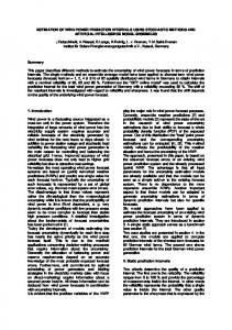
This section starts with presenting some cumulative error distributions of lateral and longitudinal RMS errors, calculated between the ground truth and the predicted paths. Next, the predictions are studied during two lane change scenarios, followed by a selection of typical cases that yield large prediction errors. Finally, the error distributions are discussed again, this time taking into account the insights gained from studying the special cases.

4.2.1

Cumulative Error Distributions

Studying cumulative error distributions helps analyzing the overall performance of a path prediction algorithm. Further, the performance can be compared to that of other models. In order compare the performance of the proposed model with other models, the error distributions of three additional models will also be shown. These models are the CA model, the LC model and the CLP model. The CA model is a kinematic motion model assuming constant acceleration, as described in chapter 2. The LC model and the CLP model are both similar to the proposed model, except for that they do not consider the driver intention. Therefore, the final position will always be in the object’s current lane. While the LC model assumes the final lateral position to be in the lane center, the CLP model assumes that the final lateral position is equal to the initial lateral position. The error distributions shown are based on the lateral and longitudinal errors between the ground truth and the actual path. From Fig. 4.1a it is seen that the longitudinal errors, considering all data, are almost identical for the compared prediction algorithms. This can be expected since they all assume constant longitudinal acceleration. When comparing the lateral errors, as displayed in Fig. 4.1b, it can be seen that the models using road structure information on average yield more accurate predictions 38


than the CA model. Moreover, it is seen that the CLP model is slightly better than the LC model, which in turn is slightly better than the proposed model. Fig. 4.1c displays the lateral error distributions when the models are compared within a time window of 6 s. centered around approximate object lane changes. It can be seen that the CA model yields the most large errors, but also that the difference between the CA model, the LC model and the proposed model is smaller than in Fig. 4.1b. Further, the proposed model performs slightly better than the LC model, but slightly worse than the CLP model. If the same time window is studied, but only for cases when the intention is to change lane, Fig. 4.1d shows that the proposed model improves on the LC model for small errors, but that it also has more large errors. Furthermore it is seen that the CA model makes the most accurate predictions for small errors but that the LC model has fewer large errors. In order to better understand the error distributions, two lane change scenarios as well as a few cases of misclassifications will be analysed.

4.2.2

Predictions During Two Actual Lane Changes

For each of the lane changes, two photos are displayed, showing the actual scenario before and after the lane change. The course of events is then analyzed by viewing plots of the predictions. All predictions are displayed in relation to the lane marker estimates. A legend for the algorithms displayed in the lane change scenarios is found in Fig. 4.2. This legend is also valid for the scenarios discussed in section 4.2.3.

4.2.2.1

Constant acceleration Constant lateral position Lane center Proposed model Ground truth

Figure 4.2: Legend for the path prediction algorithms

Left Lane Change

The first lane change scenario, as perceived by the on board camera, can be seen in Fig. 4.3a and 4.3b. In Fig. 4.4a it can be seen that the lane change is predicted 2.3 s. before the the lane markers are crossed. The intention, however, switches back to keep lane again 2 s. before the lane change, as seen in Fig. 4.4b. Just before the lane change is detected again, Fig. 4.4c displays how the algorithms using road structure information generate paths that follow the road geometry, while the CA model predicts a path following the actual path. When the lane change is detected the proposed algorithm predicts a path closely following the ground truth, as seen in Fig. 4.4d. As the vehicle changes lane the proposed model’s prediction becomes 39


1 Cumulative error distribution

Cumulative error distribution

1 0.9 Lane center Constant lateral position CA Proposed model

0.8 0.7 0.6 0.5

2

4 6 Lgt error [m]

0.9

0.7 0.6 0.5

8

Cumulative error distribution of mean longitudinal errors (a)

2

3 4 Lat error [m]

5

6

Cumulative error distribution of mean lateral errors 1 Cumulative error distribution

Cumulative error distribution

1

(b)

1 0.9 Lane center Constant lateral position CA Proposed model

0.8 0.7 0.6 0.5

Lane center Constant lateral position CA Proposed model

0.8

1

2

3 4 Lat error [m]

5

Lane center Constant lateral position CA Proposed model

0.8 0.7 0.6 0.5

6

Cumulative error distribution of mean lateral errors when the starting time of the prediction is either within 3 s. before or after a lane change (c)

0.9

1

2

3 4 Lat error [m]

5

6

Cumulative error distribution of mean lateral errors when the starting time of the prediction is either within 3 s. before or after a lane change and the estimated intention is to change lane (d)

Figure 4.1: Cumulative error distributions. equal to that of the LC model. Fig. 4.4f displays that as the object approaches the lane center, the lateral acceleration decreases causing the CA model to predict that the object continues towards the next lane. The decreasing lateral acceleration also makes the CLP model’s prediction less inaccurate. Furthermore, the lane marker estimates indicate a large road curvature, although it can be seen from the camera images that this is not the case. This negatively affects the accuracy of the path generation of the models utilizing road structure information, by providing a final lateral position that is not in the center of the actual road. 4.2.2.2

Right Lane Change

The second lane change scenario can be seen in Fig. 4.5a and 4.5b. Before the estimated intention is to change lane the same behavior as for the first lane change is seen, namely that the road structure based models assume that the vehicle will follow the road geometry while the CA model assumes a straight path, as can be seen in Fig. 4.5c. When the intention becomes correctly estimated, as shown in Fig. 4.5d, the proposed algorithm yields a more accurate path prediction. This lane change has however a slower lateral motion than the one shown in Fig. 4.4 and 40


The intention is estimated as left lane change 1.8 s. before the vehicle changes lane. The vehicle that is changing lane is the second closest one. (a)

The vehicle has changed lane. (b)

Figure 4.3: A left lane change seen from the camera. because of the tuning of the path generation the path is not as accurately described in this case. The instance before the vehicle crosses over into the new lane, Fig. 4.5e reveals that the model assuming the lane center as final position is the least accurate, followed by assuming constant lateral position. Also in this case the lane marker estimates show an incorrectly curved road, but in contrast to the other lane change it improves the prediction. However, this kind of improvement can not be trusted to generalize well.

4.2.3

Typical Scenarios That Give Large Prediction Errors

Although the proposed algorithm does indeed improve on the LC model in the lane change scenarios shown above, this is not mirrored in the error distributions. Therefore, it is of interest to find the sources of the large errors during lane changes. To do that some typical cases are shown and discussed. The actual scenario is shown as a series of images and a legend for the algorithms is found in Fig. 4.2. Fig. 4.6a shows a vehicle that is moving close to the lane marker estimates. The SVM predicts this as a lane change, but since the object does not follow a lane change trajectory the prediction goes wrong. By looking at the camera images shown in Fig 4.6b and 4.6c it is seen that the object is in fact keeping the lane and that the reality does not look like the plot. Fig. 4.7a displays the path of an object that changes lane. However, it suddenly changes direction and drives back again, after which it closely follows the lane markers. By examining the actual course of events shown in Fig. 4.7b - 4.7d, it is seen that the object is overtaken by the host vehicle. However, it is in fact making a lane change. This means that the prediction is correct, but not the ground truth. Fig. 4.8a displays an object making a lane change before quickly changing its lateral velocity. The camera images in Fig. 4.8b - 4.8d reveal that the object is making a lane change and is then overtaken by the host vehicle, similar to the case shown in 41


Fig. 4.7.

0 0 −1 Lateral position [m]

Lateral position [m]

−1 −2 −3 −4 −5

−3 −4 −5

−6 0

−2

20

40 60 80 Longitudinal position [m]

100

−6 0

120

The lane change is detected 2.3 s. before the vehicle crosses the lane markers (a)

20


100

120

The intention changes back again 2 s. before the lane change (b)

0 0 −1 Lateral position [m]


−1 −2 −3 −4 −5

−4

−6 20


100

120

Just before the intention changes (c)

0

20


100

120

The intention is again estimated as left lane change 1.8 s. before the lane markers are crossed (d)

2

2

1

1 Lateral position [m]


−3

−5

−6 0

−2

0 −1 −2

0 −1 −2 −3

−3 −4 0

20


100

120

Right after the vehicle has changed lane (e)

Figure 4.4: A left lane change 42

0

20


100

120

The lane marker estimates cause the final position to be erroneously biased (f)


Just before the lane change is detected (a)

(b)

The lane change is detected

−2 −2 Lateral position [m]


−3 −3

−4

−5

−4 −5 −6 −7

−6 −8 0

20


100

120

Just before the lane change is detected (c)

0

(d)

20


100

120

The lane change is detected

−2 −4

−4



−3

−5 −6 −7 −8

−5 −6 −7 −8

−9 0

20


100

120

Right before the lane markers are crossed (e)

0

20


100

120

(f) The lane markers are crossed

Figure 4.5: A right lane change

4.2.4

Error Distributions Revisited

The paths shown in Fig. 4.6 - 4.8 can be understood by considering that the sensors used to make the measurements of the objects, namely the radar and the camera, do not have a 180◦ view of the surroundings. Instead, they both look forward at different angles. In all the shown cases with poor ground truth, it seems to be the case that the object’s rear end disappears from the camera view. The rear end of the object is used to identify the position of the object, which means that in these cases only the radar sees the object. Hence less information can be used to estimate the state of the object, which in turn means that the quality of the object information 43



−2 −4 −6 −8 −10 −12 0

20


100

120

(a)

(b)

(c)

Figure 4.6: A case where the object is not behaving according to the ground truth −2 −3 Lateral position [m]

−4 −5 −6 −7 −8 −9 −10 −11 0

20


100

120

(a)

(b)

(c)

(d)

Figure 4.7: An object makes a lane change and is then overtaken by the host vehicle

44


−1


−2 −3 −4 −5 −6 −7 −8 −9 −10 0

20


100

120

A seemingly strange object maneuver

(b)

The object is changing lane

(d)

(a)

(c)

The prediction starts

The host vehicle is catching up on the object

Figure 4.8: An object makes a lane change and is then overtaken by the host vehicle

decreases. In cases when the camera initially sees the rear end, then the predictions might be accurate but not the ground truth, as seen in Fig. 4.8, due to that the state information is initially accurate. Since it is often the case that vehicles pass close to the host vehicle, and thus are not seen by the camera, many of the errors are caused by improper ground truth and/or measurements, which means that the error distributions do not properly describe the performance of the predictions. Thus, in order to properly evaluate the performance of the algorithm, the evaluation procedure should be run again, using only cases when both the camera and the radar can see the object. However, there was not time to rerun the evaluation within the scope of the thesis since this was discovered late. It is however possible to say a few things regarding the error distributions. In cases when the ground truth states that the vehicle is driving on the lane markers, such as shown in Fig. 4.6a, the CLP model can accurately describe the ground truth, while at the same time all the other compared models yield large errors. This means that in the error distributions of object lane changes shown in Fig. 4.1d, the CLP model appears to be better than it is due to that it is able to describe the cases with noisy sensor data more accurately than the other models. Both the CLP model and the LC model yield small errors when a vehicle is following the lane center but the CLP model also gives small errors when a vehicle is following a path with constant offset 45


from the lane center. This can explain why the CLP model is the best model on average. Possibly, there are cases with poor state estimations also here. Further, it can be said that the largest errors of the CLP model are due to a bug in the code which occasionally places the final lateral position on the wrong side of the lane, as seen in Fig 4.8a. Although the performance of the proposed model can not be properly analysed from the shown error distributions, it seems to be the case that the proposed model improves on the LC model, based on the displayed lane change scenarios. Also, Fig. 4.1d shows that the proposed model clearly improves on the LC model for small errors. Regarding the large errors, although they are probably sometimes caused by misclassifications, these cases are hidden among the cases with noisy data. Examples similar to the one shown in Fig. 4.6a could explain why the distribution of the LC model gives more accurate predictions than the proposed model in such cases.

4.3

Parameters

It is possible to tune several of the parameters of the implementation in a better way. A discussion regarding this follows.

4.3.1

SVM Parameters

The classification accuracy of the SVM depends on the features as well as the parameters C and γ. Since these parameters have been tuned empirically, it is likely possible to improve the tuning. In [12], an approach to find suitable parameter values for C and γ is to perform grid searches where different parameter combinations are evaluated, and cross-validation is employed for each combination.

4.3.2

Window Size

Including past measurements in the feature vector helps the SVM detect temporal patterns in the data, such as a decrease or increase in the lateral position. As an example, utilizing only the latest measurement of the lateral position as a feature can be considered. Then the SVM could only find threshold values to use for the classification. This would lead to high noise sensitivity, since a single outlier could cause the threshold value to be passed. Bearing in mind the same line of argument, it could be advisable to use windows also for the similarity features. In Tab. 4.1 - In Tab. 4.3 it is seen that the similarity features are not able to predict lane changes with as high accuracy as the lateral position features. Furthermore, they only slightly improve the prediction accuracy when used together with the lateral position features. However, a windowed version of the similarity features would be able to resist outliers and find patterns in the data which might enhance the classification ability further. 46


4.3.3

Down Sampling

The measurements were on average updated every 0.025 s. Since the motion of road vehicles does not change much in such a short time, it might be possible to use only a subset of all measurements without loosing accuracy. This would mean shorter feature vectors and hence also shorter time needed for training and evaluation. Shorter training time is especially useful when searching for the optimal parameters.

4.3.4

Labelling Horizon

It is not obvious why to decide the labels with a fixed time threshold since lane changes obviously do not take equally long time. Reasons behind this method are that it is easy to implement and that it has been used for lane change detection with good results in [25]. From studying the features in Fig. 3.4 and 3.5 an intuition can be gained, namely that a shorter labelling horizon gives a higher prediction accuracy at the cost of making the classifications regarding lane changes later, while a longer horizon can make it hard to find enough patterns in the data to be able so accurately make classifications. Thus the fixed threshold has to be a trade off between classification accuracy and making early predictions. The threshold value of 1.8 seconds was chosen empirically, but a more thorough approach could be to examine how different labelling horizons affect the prediction accuracy. Alternatives to using a fixed labelling horizon would be to manually label the data or to use an algorithm, e.g. an unsupervised learning algorithm, that finds a pattern to put the labels. However, manually labelling the data is time consuming for large amounts of data, and furthermore does not guarantee that the labels will be set accurately. As of using an unsupervised learning algorithm, that would be another project.

4.3.5

Similarity Features

Although the similarity features prove to be able to predict lane changes in the training data, they could be varied in several ways, including the placement of the grid points and the motion model.

4.3.6

Path Generation

The time penalization parameter, α, that is used to generate paths has to be tuned to estimate trajectories accurately. A problem in tuning α is that lane change trajectories can differ depending on several factors, such as the driver and the scenario. Possibly, probabilistic methods could be utilized to tune the parameter and express the uncertainty of the trajectory. In the combined prediction, the weights are obtained from a sigmoid function, due to its monotonous and continuity properties. However, the parameters a and b need to be tuned to obtain the best combined trajectory. Statistical methods can be utilized to tune the parameters depending upon the uncertainty between the road structure information and the object data. 47


4.4

Road Structure Information

The proposed algorithm depends on road structure information in several ways. First, when calculating the lateral position feature. Second, the similarity features use road structure information for placing the grid points and third, road structure information is used to decide the final lateral position. Therefore, inaccurate road structure information will decrease the accuracy of the features as well as the generated path. Since most of the data in the used data sets does not contain accurate road structure information up until the point where the final position is placed, the constraints on which data to use were softened to get data to evaluate the algorithm on. However, this means that most of the time, the predictions are not as accurate as they could be. Further, it means that the proposed algorithm would benefit from using additional information, such as electronic horizon data, to improve the the perception of the world.

4.5

Motion Models

The CA model, which is used both in the similarity features and in the path generation, was chosen for its simplicity. Furthermore, even though the data sets that were used contain mixed road types, the constraints used to select data for evaluation resulted in that the data that was actually used is mostly from highways or larger roads where the curvature is low. This means that the CA model is suitable. However in curved roads a more advanced motion model, such as the CYRA model, or even a mixture of different models for different scenarios, might be a better choice. A problem with using more advanced motion models on object data could be that the yaw rate and curvature estimations are not as accurate as for the host vehicle. This problem could be tackled by using a measure of confidence for the state estimation parameters of the objects to be able to use these measurements when they can be trusted.

4.6

Choice of Multiclass Method

As mentioned the choice of multiclass extension for the support vector machine is the one-versus-one classifier. Although a thorough comparison has not been made between different approaches, this choice has resulted in high classification accuracy on the host data. Furthermore, it can be said that the drawback of long training and execution times does not provide a problem since only a few classes are used.

4.7

Flipping Intention

As seen in 4.4 the intention estimation can be uncertain prior to a lane change. This might be explained by that the feature vectors for keep lane and lane change intentions are similar in a certain region before a lane change. Furthermore, the SVM always makes a classification even if the feature vector is really close to the 48


decision boundary. There are, however, several approaches towards giving the SVM a probabilistic output. Doing so might be helpful in order to find out when the intention estimation is uncertain.

4.8

More Intentions

The currently used intentions can not describe all object behaviors. For instance vehicles sometimes choose connecting roads, stop or cut corners. If the set of intentions in enlarged, then the proposed features can be applied to intentions such as choosing a connecting road since they provide comparisons between objects’ state and the road geometry. However, in order to extend the number of classes, feature vectors belonging to the additional classes must be identified and labelled. Since the only such information contained in the current data set is lane change flags, increasing the number of classes requires either a more sophisticated method of labelling or more flags marking interesting events. Another challenge is that the road structure information in the used data set is accurate enough mostly in highway scenarios. More accurate road structure information, not only during highway scenarios, would allow making predictions in a larger variety of scenarios. One way of achieving this is to use electronic horizon data. Electric horizon data would also simplify the labelling.

49


50

5 Conclusions and Future Work In this thesis a framework for predicting the paths of road participants has been presented. The driver intention is estimated with support vector machines, that combine information about the vehicle’s lateral position and motion in relation to the road, and is then included in the path prediction. The path prediction consists of a combination of a constant acceleration (CA) model prediction and a long term prediction that assumes that the vehicle follows the road, where the final lane is determined from the driver intention. These predictions are combined using a sigmoid function, such that the CA model prediction is trusted more in the beginning of the trajectory and the long term prediction more towards the end of the trajectory. The algorithm has been tested in lane change scenarios and the test results show that the algorithm can correctly predict lane changes and further, that the path prediction is improved by the driver intention in lane change scenarios. However, the overall evaluation of the framework does not reflect the actual performance since the evaluation data contain several cases of inaccurate state estimations due to that the vehicle was not in range of the sensors. Therefore, a new evaluation, excluding these cases, should be performed in order to understand the actual performance of the system. Future work on the algorithm could also include using more advanced motion models than the CA model in cases when the road has large curvature. There are several challenges in improving the proposed algorithm. First, it has been observed that the driver intention can alternate between two states. This behavior was observed shortly before the changes. A possible explanation is that the feature vectors in these cases are close to the decision boundary. This means that the predictions are uncertain. Therefore, an estimate of the confidence of the intention estimation could be helpful when addressing this problem. Such a measure could be helpful also for detecting and handling misclassifications. Second, the quality of the road structure information is most of the time not high enough for the proposed algorithm. Therefore, the framework would benefit from using electronic horizon data. Third, there are several parameters to tune in the SVM, when creating the features and for generating the path prediction. The parameter tuning in this thesis has been done empirically and it is therefore likely that the tuning can be improved. Finally, more intentions could be included to handle cases that can not be described by lane changes, e.g. when the vehicle stops or drives onto a connecting road. The current limitation for this is to find cases in the log data that can be used for training. Utilizing electronic horizon data would be a great help in finding scenarios containing different types of intentions. 51

5. Conclusions and Future Work

52

Bibliography [1] Global plan for the decade of action for road safety 2011-2020. [2] European new car assessment programme 2020 roadmap. March 2015. [3] Polychronopoulos A, Tsogas M, Amditis AJ, and Andreone L. Sensor fusion for predicting vehicles’ path for collision avoidance systems. IEEE Trans on Intell Transportation Syst, page 8(3):549–562, 2007. [4] Morris B, Doshi A, and Trivedi M. Lane change intent prediction for driver assistance: on-road design and evaluation. Proc. IEEE Intelligent Vehicles Symposium, page pp 895–901, 2011. [5] C. Ben-Hur and J. Weston. A user’s guide to support vector machines. Technical report, Colorado State University and NEC Labs America. [6] C. M. Bishop. Pattern Recognition and Machine Learning. Springer. [7] Mattias Brännström. Decision-making in automotive collision avoidance systems. Chalmers University of Technology, ISBN: 978-91-7385-618-8.- 146 pp. [Doctoral thesis], 2011. [8] Hermes C, Wohler C, Schenk K, and Kummert F. Long-term vehicle motion prediction. Proc. IEEE intelligent vehicles symposium, page pp 652–657, 2009. [9] Laugier C, Paromtchik I, Perrollaz M, Yong M, Yoder JD, Tay C, Mekhnacha K, and Negre A. Probabilistic analysis of dynamic scenes and collision risks assessment to improve driving safety. IEEE Intell Transportation Syst Mag, page 3(4):4–19, 2011. [10] Tay C. Analysis of dynamic scenes: application to driving assistance. PhD thesis, Institut National Polytechnique de Grenoble, France, 2009. [11] Lin C-F, Ulsoy AG, and LeBlanc DJ. Vehicle dynamics and external disturbance estimation for vehicle path prediction. IEEE Trans on Control System Technology, page 8(3):508–518, 2000. [12] C.-C. Chang C.-W. Hsu and C.-J. Lin. A practical guide to support vector classification. Technical report, National Taiwan University. 53

Bibliography

[13] Buzan D, Sclaroff S, and Kollios G. Extraction and clustering of motion trajectories in video. Proc. international conference on pattern recognition, pages vol. 2, pp 521–524, 2004. [14] P. Datseris. Mce 263 lecture notes: Normal - tangential. University Lecture notes, 2015. [15] P. Domingos. A few useful things to know about machine learning. Technical report, University of Washington, Department of Computer Science and Engineering. [16] Marco Dozza. Lecture notes-active safety: Introduction. Chalmers University of Techology, Sweden, 2014. [17] Aoude GS, Luders BD, Lee KKH, Levine DS, and How JP. Threat assessment design for driver assistance system at intersections. Proc. IEEE intelligent transportation systems conference, page pp 25–30, 2010. [18] Berndt H, Emmert J, and Dietmayer K. Continuous driver intention recognition with hidden markov models. Proc. IEEE intelligent transportation systems conference, page pp 1189–1194, 2008. [19] Veeraraghavan H, Papanikolopoulos N, and Schrater P. Deterministic samplingbased switching kalman filtering for vehicle tracking. Proc. IEEE intelligent transportation systems conference, page pp 1340–1345, 2006. [20] Tan H-S and Huang J. Dgps-based vehicle-to-vehicle cooperative collision warning: engineering feasibility viewpoints. IEEE Trans on Intell Transportation Syst, page 7(4):415–428, 2006. [21] A. Houenou, P. Bonnifait, V. Cherfaoui, and W. Yao. Vehicle trajectory prediction based on motion model and maneuver recognition. Intelligent Robots and Systems (IROS), 2013 IEEE/RSJ International Conference on, 2013. [22] Hillenbrand J, Spieker AM, and Kroschel K. A multilevel collision mitigation approach: situation assessment, decision making, and performance tradeoffs. IEEE Trans on Intell Transportation Syst, page 7(4):528–540, 2006. [23] Huang J and Tan H-S. Vehicle future trajectory prediction with a dgps/insbased positioning system. Proc. American control conference, page pp 5831–5836, 2006. [24] Murphy KP. Dynamic bayesian networks: representation, inference and learning. PhD thesis, University of California at Berkeley, USA, 2002. [25] P. Kumar, M. Perrollaz, S. Lefevre, and C. Laugier. Learning-based approach for online lane change intention prediction. IEEE Intelligent Vehicles Symposium, Gold Coast, Australia, 2013. [26] S. Lefevre, D. Vasquez, and C. Laugier. “a survey on motion prediction and risk assessment for intelligent vehicles. Robomech Journal, pages 1(1),1–14, 2014. 54

Bibliography

[27] Brännström M, Coelingh E, and Sjöberg J. Model-based threat assessment for avoiding arbitrary vehicle collisions. IEEE Trans on Intelligence Transportation Systems, page 11(3):658–669, 2010. [28] H. M. Mandalia and D. D. Salvucci. Using support vector machines for lanechange detection. Hum. Factors and Ergonomics Soc. 49th Annu. Meeting, Orlando, FL, 2005. [29] Kaempchen N, Weiss K, Schaefer M, and Dietmayer KCJ. Imm object tracking for high dynamic driving maneuvers. Proc. IEEE intelligent vehicles symposium, page pp 825–830, 2004. [30] A. Ng. Cs229 lecture notes: Support vector machines. University Lecture notes, Nov 2012. [31] N. J. Nilsson. Introduction to machine learning. 1998. [32] Pepy R, Lambert A, and Mounier H. Reducing navigation errors by planning with realistic vehicle model. IEEE intelligent vehicles symposium, page pp 300–307, 2006. [33] Ammoun S and Nashashibi F. Real time trajectory prediction for collision risk estimation between vehicles. Proc. IEEE intelligent computer communication and processing, page pp 417–422, 2009. [34] Atev S, Miller G, and Papanikolopoulos NP. Clustering of vehicle trajectories. IEEE Trans on Intell Transportation Syst, page 11(3):647–657, 2010. [35] J. Schlechtriemen, A Wedel, J. Hillenbrand, G. Breuel, and K.D.Kuhnert. A lane change detection approach using feature ranking with maximized predictive power. Intelligent Vehicles Symposium Proceedings, 2014 IEEE, pages 108–114, 2014. [36] R. Schubert, E. Richter, and G. Wanielik. Comparison and evaluation of advanced motion models for vehicle tracking. International Conference on Information Fusion, Cologne, Germany, Jul 2008. [37] Batz T, Watson K, and Beyerer J. Recognition of dangerous situations within a cooperative group of vehicles. Proc. IEEE intelligent vehicles symposium, page pp 907–912, 2009. [38] Streubel T and Hoffmann KH. Prediction of driver intended path at intersections. Proc. IEEE Intelligent Vehicles Symposium, page pp 134–139, 2014. [39] Jerome Friedman T. Hastie, Robert Tibshirani. The Elements of Statistical Learning. Springer. [40] Hu W, Xiao X, Fu Z, Xie D, Tan T, and Maybank S. A system for learning statistical motion patterns. IEEE Trans on Pattern Anal Mach Intell, page 28(9):1450–1464, 2006. 55

Bibliography

[41] W. Yao, H. Zhao, F. Davoine, and H. Zha. Learning lane change trajectories from on-road driving data. IEEE Intelligent Vehicles Symposium, Alcala de Henares, Spain, June 2012. [42] Z. Zhang, K. Huang, and T. Tan. Comparison of similarity measures for trajectory clustering in outdoor surveillance scenes. Proc. IEEE Intell Conf. Pattern Recognition, 2006.

56

Mixed Driver Intention Estimation and Path Prediction Using Vehicle

Mixed Driver Intention Estimation and Path Prediction Using Vehicle

Suggest Documents

Estimation of Driver Distraction Using the Prediction ...

Driver Identification Using Vehicle Telematics Data

Control and path prediction of an automate guided vehicle

Control and path prediction of an automate guided vehicle

Vehicle Tracking and Speed Estimation using

Prediction of Driver Intended Path at Intersections - IEEE Xplore

Vehicle Full-State Estimation and Prediction ... - Semantic Scholar

mixed integer programming for multi-vehicle path planning - CiteSeerX

mixed integer programming for multi-vehicle path planning - CiteSeerX

3D Pose Estimation of Front Vehicle Towards a Better Driver

path prediction and path diversion identifying ... - CiteSeerX

Difficult-Path Branch Prediction Using Subordinate Microthreads ...

driver intention to use electric cars using technology ... - ARPN Journals

Pedestrian Path Prediction Using Body Language Traits

Difficult-Path Branch Prediction Using Subordinate Microthreads ...

Using vehicle monitoring technology and eco-driver training to reduce ...

path radiance estimation using reflectance measurements ... - ISPRS

path radiance estimation using reflectance measurements in

Queue Length Estimation using Conventional Vehicle ...

Vehicle Velocity Estimation using Modular Nonlinear Observersâ

vehicle acceleration estimation using smartphone-based sensors

Vehicle Speed Estimation Using a Monocular Camera

A Conceptual Framework and Intention Prediction Algorithm

ESTIMATION OF WIND POWER PREDICTION INTERVALS USING ...

Mixed Driver Intention Estimation and Path Prediction Using Vehicle