2014 IEEE Intelligent Vehicles Symposium (IV) June 8-11, 2014. Dearborn, Michigan, USA
Prediction of Driver Intended Path at Intersections Thomas Streubel1 and Karl Heinz Hoffmann2
The key aspect remains in the situation assessment. This is necessary to derive adequate actions or possible warning strategies. Next to sensing and situation analysis that combines the perception of the environment and the interpretation of detected objects, it is essential to predict the dynamics of the scene. The driver’s intention is of high interest in particular. This way, a possible conflict can be identified in advance giving enough time for intervention strategies. For example, when two vehicles are approaching from different sides, a conflict may arise only dependent on the direction of their path (see Figure 1).
Abstract— The complexity of situations occurring at intersections is demanding on the cognitive abilities of drivers. Advanced Driver Assistance Systems (ADAS) are intended to assist particularly in those situations. However, for adequate system reaction strategies it is essential to develop situation assessment. Especially the driver’s intention has to be estimated. So, the criticality can be inferred and efficient intervention strategies can take action. In this paper, we present a prediction framework based on Hidden Markov Models (HMMs) and analyze its performance using a large database of real driving data. Our focus is on the variation of the model parameters and the choice of the dataset for learning. The direction of travel while approaching a 4-way intersection is to be estimated. A solid prediction is accomplished with high prediction rates above 90% and mean prediction times up to 7 seconds before entering the intersection area.
I. I NTRODUCTION The development of Advanced Driver Assistance Systems (ADAS) is proceeding towards automated driving [1]. Though, while this step is nearly reached for highway traffic, the development of ADAS is just evolving for urban environments. Here, intersections seem to be particularly crucial considering the high number of accidents and traffic jams in rush hour. The urbanization will amplify this problem even further. In Germany, the majority of accidents with personal injuries took place on urban roads with a proportion of 69% in 2012 [2]. Hereof, 43% were caused by either turning on or crossing an intersection. Complex intersection scenarios are demanding on cognitive abilities of the driver which leads to an increased error rate. In these situations assistance is most desirable. However, the complexity of situations occurring and the high number of possible scenarios are challenging and require adequate situation analysis and recognition approaches. Besides, dangerous situations may arise from vehicles or pedestrians out of sight that visual based sensors cannot detect. Accordingly, robust object detection is required to recognize the situation correctly. The visibility restraints are typical for urban scenarios and can be overcome with Vehicle-to-Vehicle (V2V) and Vehicle-to-Roadside (V2R) communication. Both combined are known as V2X. This exchange of information is feasible particular at intersections to detect oncoming vehicles from different directions that are not yet in the line of sight. 1 Thomas Opel AG,
Fig. 1. Example of path conflict (left) and no conflict (right) of two vehicles approaching an intersection only dependent on the driving direction of the ego vehicle (blue/south)
A. Related Work There is a variety of approaches to accomplish such a prediction. The uncertainty of the driver’s intention calls for probabilistic methods such as Bayesian networks [3], [4], [5] or neuronal networks [6], [7]. There are other approaches using clustering and classification algorithms to estimate motion patterns [8], [9], [10]. For the prediction of lane changes, there are even mathematical models utilized [11]. The dynamic of an intersection situation is highly variable. Hidden Markov Models (HMMs) are a capable method to model dynamic stochastic processes. It is widely used in different fields, where probabilistic system states occur, such as speech recognition or even biological simulation [12]. In the automotive area, there have been approaches to use HMMs for driver behavior recognition [13]. Thereby, a system was introduced to predict the turning intention at a Tshaped intersection using only the steering angle. Also, traffic light violation behavior was estimated with this method [14]. Another approach was using linear Hidden Markov Models to determine the driver intended direction (left or right) at an intersection [15]. Again, the steering angle was used as single sensor input. Since the steering is the last action of many when turning at an intersection, better results can be accomplished involving additional vehicle information such
Streubel is with Advanced Technology, Adam IPC S4-01, D-65423 Ruesselsheim, Germany
[email protected] 2 Karl
nitz
Heinz Hoffmann is with Institute of Physics, ChemUniversity of Technology, D-09107 Chemnitz, Germany
[email protected] 978-1-4799-3637-3/14/$31.00 ©2014 IEEE
134
𝐴
𝐴
as velocity. In [16], HMMs were used for estimation vehicle states and maneuver prediction. In this paper, we utilized Hidden Markov Models in a similar way. However, we further investigated, if there are optimal model parameters and how the performance of the prediction can be improved by a larger learning database.
qt-1
𝐵
B. Hidden Markov Models
Ot-1
A HMM is a stochastic model which describes a dynamic process through two random processes (Markov Chains). We give a brief introduction in the following. Further details are found in the tutorial by Rabiner [17]. One of those processes is hidden, giving the method its name, and represents the state transition of the system. Meanwhile, the second one is emitting observations in each time step. The Markov attribute of the system state process is the restriction indicating the model character and representing the uncertainty of the process. The number of system states is N and determines the system’s degree of freedom. It is one parameter that is varied in our evaluation. The possible system states are S = (S1 , ..., SN ), while the sequence q = (q1 , ..., qT ) in discrete time steps t is a Markov Chain of the length T . While this is hidden, the observation sequence O = (O1 , ..., OT ) results by emitting a certain symbol R = (R1 , ..., RM ) each time step. Here, M is the number of discriminable symbols each referencing to a part of the defined state space of measurements. Mathematically, a HMM is described by the transition matrix A, the observation matrix B and the starting distribution π. Last is of less importance in our application, since we are more interested in the progress than in the starting state. The way the system changes between hidden states in discrete time steps t is described as
𝐴 qt
qt+1
𝐵 Ot
𝐴
𝐵 Ot+1
Fig. 2. Trellis structure of a HMM with hidden state sequence q and observation sequence O accordingly
Learning: What are the optimal model parameters that maximize the probability for an existing observation sequence O? Here we are looking for the parameters of the HMM λ(A, B, π) where P (O|λ) is the highest. Representation: What is the probability for an existing observation sequence O being created by a given HMM? Here we have to calculate P (O|λ). The latter can be solved with the forward algorithm. However, solving the learning problem is more complicated since there is no known analytical algorithm. A common numerical solution gives the Baum Welch algorithm, which is a type of Expectation-Maximization-algorithm (EM). First, we determine initial values λ0 for the HMM parameters. This is usually done by random choice or manually, if there is a priori knowledge about the model. The choice of starting values has an influence on the outcome. Next, the expectation step where the expected frequency of system states and translations are calculated with the initial parameters. These values lead to an adaption of the model parameters which is the maximization step. Afterward, the new model parameters can be used again to calculate new frequencies and translations and so on (see Fig. 3). Baum and Welch have proven that the probability of the sequence being created ¯ is the same or higher than with the by the new model λ previous parameters. Furthermore, this algorithm converges quickly to a local optimum. Thus, it is recommended to run the algorithm several times with different starting conditions, not only randomized but also scattered evenly through the probability space.
A = {aij } ⇒ aij = P (qt+1 = Sj |qt = Si ) So, A is a N ×N matrix. The probability of an observation Rj at the time t while in state Si is determined by the observation matrix B of size N × M . B = {bij } ⇒ bij = P (Ot = Rj |qt = Si ) Here, the hidden state as well as the observation are discrete. At last, the distribution of the first state is defined by the vector πi = P (q1 = Si ). So, a discrete Hidden Markov Model λ is defined by the above explained parameters. Graphically, the process can be displayed in a Trellis structure as shown in Fig. 2. In our application, the observation symbols are a set of vehicle data. However, the hidden states are an abstract situation status and could be interpreted as steps in the decision process of the driver. There are two essential processes necessary to work with HMMs. First the model parameters are determined. Commonly, this is achieved by a learning procedure which requires a labeled training set of data. To use it in a prediction framework an unknown dataset is to be related to the model. There, it is tested how well the model represents the data. These two procedures are answering the following questions.
„Calculate expected state transition and observation values“
𝜆0
Expectation-Step
𝑃(𝑂|𝜆) ≥ 𝑃(𝑂|𝜆)
Maximization-Step „Adaption of model parameters“
Fig. 3.
135
Baum Welch algorithm procedure
II. DATA A NALYSIS
The turning signal was not considered intentionally. On the one side, there is a small possibility of misuse; on the other side in multi-lane intersections the turn signal can indicate a lane change rather than the intention to turn. Besides, it is easier adaptable relying on basic dynamic parameters. The average approaching speed is displayed in Fig. 5. Hereby, only vehicles on the main road were considered. At a distance to intersection of 100 meters, the velocities are still at a similar level independent on the direction of travel. While driving straight through the intersection, the velocity is kept steady at about 50 km/h on average; which is the speed limit for inner-city traffic in Germany. Both turning events show a decrease in the vehicle speed. When turning left, the velocity graph starts below the others. The speed reduction is more intense down to 22 km/h entering the intersection, while the average speed for turning right amounts to 32 km/h.
Using HMM requires a certain amount of data for learning and testing. We had access to the database of the ”Safe and Intelligent Mobility Test Field Germany” (simTD ) project, which was a large-scale field test for V2V communication [18]. Here, it has been made use of data from two days of testing, conducted on the simTD test site in Friedberg, Germany. The data was recorded for project related V2V applications. About 30 test drivers participated with vehicles of different types. A complex 4-way intersection was installed at the premises (see Fig. 4). The traffic light had been deactivated for the experiment. Therefore, the traffic signage indicated the right of way for vehicles coming from east and west. Accordingly, the north and south branches are side roads, where drivers have to yield. There were no further instructions whether to turn or go straight at the intersection. So, all vehicles were moving simultaneously and undirected on the test area and through the intersection. Here, we concentrated on the intersection approaches on the main road. This data will be applied in the prediction framework. For further details especially blinker usage and gear shift behavior, we refer to the results of the in-depth analysis [19].
Average speed [km/h]
60 50 40 straight turn right turn left
30 20 100
183
Fig. 5.
931 796
main road
80
60 40 Distance to intersection [m]
20
0
Average velocity approaching on main road
The acceleration can be estimated contemplating the velocity graphs. As expected, there is no deceleration when going straight (see Figure 6). Neither the right nor the left turning sequences start with a deceleration on average. For about 30-40 meters, there is no driver induced reduction but rather a slight deceleration due to coasting. Afterwards, the driver brakes, showing a noticeable deceleration. Here, the average acceleration for left turning sequences decreases more intensively to a minimum of about -2 m/s at a distance of about 18 meters to the intersection. Since the oncoming traffic can retard the left turn, the drivers seem to reduce the speed in advance to gain more time for clearance. The right turn sequences show a monotonous average deceleration up to entering the intersection. The yaw rate is examined as an indication for a turning movement. If driving straight, there is no yaw. Thus, the yaw rate in straight sequences is near zero. We determined the standard deviation over all straight sequences to distinguish them from turning sequences. Here, this threshold was found to be 0.5644 /s. The distance to intersection in turning sequences where this value is exceeded, is indicated as a vertical line in each graph in Figure 7. There it is shown, that the yawing starts earlier when turning left at a distance of about 22 meters in comparison to about 12 meters in right turning sequences. However, the deviation for left turning is noticeably higher because there were less sequences
586
Fig. 4. Intersection area at the premises of simTD test field (aerial view from Google earth) with main and side road and number of available approaching sequences for each direction
First, we retrieved all intersection approaches within 100 meters distance. This was accomplished by using differential GPS raw data, which was specified to have a mean error of about 3 meters. The intersection area was defined as the area passable by vehicles approaching from different directions, i.e. where collisions are most likely. Thus, the area of interest was determined. So, the distance to intersection, indicated in the following figures, is the distance to entering the intersection area. The data recording was harmonized by a specific simTD protocol. However, some datasets were incomplete or asynchronous and have been discarded. Considering basic vehicle dynamics and comparing going straight versus turning, differences occur in the velocity, acceleration and steering angle. Unfortunately, the last one was too noisy, which is why the yaw rate was used instead. 136
is executed at least ten times with different randomized initial values, resulting in 10 different models for each direction. The one with best log-likelihood of representing the learned dataset was accepted and represents the according scenario. So, we obtain three HMMs (λlef t , λright , λstraight ). For the prediction, a sequence is selected and evaluated in each time step with each model using the forward algorithm. The resulting probabilities are compared, and the sequence is assigned the direction according to the model that it best related to. Finally, the performance of the framework is determined by the number of correctly predicted sequences and the time before entering the intersection where the prediction was correct and did not change anymore. This is referred to as prediction time in the results and has been determined by backtracking. The correct prediction is determined at the end of the sequence when it corresponds to the actual driving direction.
Average acceleration [m/s²]
1 0 −1 −2 straight turn right turn left
−3 −4 100
Fig. 6.
80
60 40 Distance to intersection [m]
20
0
Average acceleration approaching on main road
available. Conclusively, the yaw rate is a solid indication of an upcoming turning event, though it occurs close to the intersection entry giving little time for an intervention strategy.
A. Clustering vs. Gaussian Mixture The data sequences consist of adjusted, sampled data at a frequency of 10 Hz (after harmonization). However, the HMM described in subsection I-B requires a set of symbols much smaller than the sampling rate. So, symbols reoccur in different sequences of the same category and can be recognized. This can be overcome by either clustering the input data or by adjusting the HMM to handle sampled data. The latter is realized with a Gaussian mixture approach. Though, the mapping of the hidden states on the observation is now a mixture of Gaussian distributions. The observation matrix B from the discrete HMM is now split into arrays for the mean values µ b, the standard deviations σ b and the weights ω b . So, the number of model parameters increases depending on the number of mixtures. This is to be considered, since a higher number of parameters requires more learning data to get adequate results. Another approach to deal with sampled data is dividing the attributes in a discrete number of groups. Here, kmeans clustering was used to create discrete observation symbols. The advantage is that the number of clusters is defined in advanced. However, the distance measure has to be determined. Using an Euclidean distance is problematic because of the different measures and span of the attributes. Therefore, this has been overcome by scaling. An alternative would be a scale invariant distance measure such as the Mahalanobis distance. The number of clusters is identical with the number of observation symbols in the HMM and this way, is influencing the number of parameters necessary to be acquired by learning.
Fig. 7. Average yaw rate with standard deviation for left turning (left) and right turning (right) sequences on the main road
III. P REDICTION F RAMEWORK The vehicle data serves as input for the framework. The velocity, acceleration, yaw rate and distance to intersection have previously been identified as relevant data. Here, the distance is included, so some information of the position are considered inherently. Utilizing GPS data, all sequences were labeled according to their direction of approach (East, West) and direction of travel (left, right, straight). Since the sample rate was not consistent, the data frequency was adjusted to 100 ms by interpolation. This is necessary, because the time steps are equal in the HMM. Main road sequences are included only to reduce the influence of other traffic participants. Overall, the completed database consisted of 146 turning left, 411 turning right and over 1000 straight sequences. First of all, three different HMMs are introduced each for one possible direction (cf. [16]). In contrast to [15], our choice was an ergodic model approach. This leads to more parameters to be estimated, because the transition matrix A is not a sparse matrix (cf. subsection I-B). This way, the possibility to get stuck in a certain state is avoided since all states can be reached and left. This is also influencing the mean prediction time, which is desired to be as early as possible. Sequences are chosen for learning the HMM parameters using the Baum-Welch algorithm (see Fig. 3). This
B. Evaluation First, we used clustering and varied the number of symbols, size of training set and hidden states. All these variations have a noticeable effect on the recognition of the learned sequences. The evaluation is performed by testing how well the training set is recognized by the models. Afterward, the performance of the framework is tested with 137
the trained models and data sequences not used for learning. The outcome is shown in the section IV Results. The number of available sequences were unbalanced for the different scenarios. There were only a few left turning datasets compared to a higher amount of right sequences. Most of the drivers went straight on the main road. A smaller training set leads to less diversity and might be easier to map the data to its corresponding scenario. So, left and right sequences were recognized by their corresponding HMM better than straight ones. The reason is a high fluctuation in the dataset of straight scenarios. Especially, the acceleration in some sequences is deviating strongly from zero. This leads to a high prediction error. 5 hidden states, 16 symbols and 146 sequences are used as standard parameters for the learning process. The hidden states were varied between 2 and 10. The number of symbols was increased to have 3 or 4 values each dimension leading to 81 or 256 symbols respectively. Further, the training set was reduced to half (73 sequences) and quarter (36 sequences). The recognition rate for left sequences are close to 100% in all evaluation variations. Seemingly, the sequences are alike. The variation of the distance measure for clustering shows no significant change in the evaluation. However, using Euclidean distance seemed more solid with a higher average correct and earlier prediction. An increase in the number of symbols improved the recognition results. This is accomplished with a higher differentiation in the event space. With 256 centroids, 96% of the left and right sequences were recognized correctly with a mean prediction time over 7 seconds before entering the intersection area. However, 21 straight sequences (14%) were predicted mistakenly to be turning ones. The reduction of the training set led to high recognition rates. However, this effect is called memorizing and is not desirable. The models are adapted perfectly to the data, thus recognition improves but the sensitivity towards differentness decreases. This is not preferable for a prediction framework that is working with diffuse data. The evaluation was performed with a different number of hidden states. Best results were shown with 8 hidden states. Here, 88% of the straight sequences were recognized correctly with a mean prediction time of 5.7 seconds. The evaluation led to the following assumptions. A higher number of centroids results in a more accurate sampling of the data which improves the prediction. However, this requires more model parameters and increases the computing time. The memorizing effect occurs when decreasing the learning datasets. Also, the optimum number of hidden states seems to be 8.
TABLE I P REDICTION RESULTS OF DIFFERENT VARIATIONS left right straight Varying number of learning sequences 256 symbols / 5 hidden states / 36 learning seq. rel. correct prediction 100% 68% 68% mean prediction time 6.7s 5.8s 7.2s prediction time >3s TTI 75% 78% 96% prediction time 3s TTI 72% 73% 93% prediction time 3s TTI 79% 93% prediction time 3s TTI 66% 97% prediction time 3s TTI 85% 71% prediction time