MIXED-MODE DEVICE AND CIRCUIT SIMULATION S. WAGNER , T. G RASSER , S. S ELBERHERR T ECHNICAL U NIVERSITY V IENNA , AUSTRIA KEYWORDS: Device Simulation, Circuit Simulation, Oscillator
A BSTRACT: We present the motivation for mixed-mode device and circuit simulation. The possible approaches are discussed and the particular methods of the multi-dimensional device/circuit simulator M INIMOS -NT are presented. The available capabilities are demonstrated on a Colpitts oscillator and two intermediate circuits, which are matter of transient and small-signal ac simulations.
MOTIVATION Advances in the development of semiconductor devices have lead to more and more sophisticated device structures. This concerns device geometry as well as doping profiles and the combination of different materials. Due to shrinking device geometries, the models describing the device physics increase in complexity. Traditional device simulation has considered the behavior of isolated devices under artificial boundary conditions (single-mode). To gain additional insight into the performance of devices under realistic dynamic boundary conditions imposed by a circuit, mixed-mode simulations have proven to be invaluable. However, this problem is very complex and only limited solutions have been available so far. The main advantages of mixed-mode simulations are: • A calibrated device simulator can be directly employed for circuit simulations: No subsequent and often expensive parameter/model extraction is necessary. Thus, in time-to-market considerations results of many different devices are available at significantly earlier times. • It is common practice to create optimization loops consisting of process and device simulators. Controlled by various kinds of optimizers, device figures of merit (e.g., cut-off frequency f t ) trigger process variations in order to be improved. By switching the device simulator in the mixed-mode, also circuit figures of merit can be optimization targets. The major drawback in comparison to compact model approaches is the significant performance difference, since much larger equation systems have to be assembled and solved.
INTRODUCTION Over the last decades, numerous powerful circuit simulation programs have been developed. Amongst those are general purpose programs (e.g., ASTAP [1] or S PICE [2]) and special purpose programs providing highly optimized algorithms, e.g. for filter design. They have in common 36
that the electrical behavior of the devices is modeled by means of a compact model, that is, analytical expressions describing the device behavior. Once a suitable compact model is found, it can be evaluated in a very efficient way. However, this task is far from being trivial and many complicated models have been developed. Even if the behavior of the device under consideration can be mapped onto one of the existing compact models, the parameters of this compact model have to be extracted, which is obviously a cumbersome task. The BSIM 4.4.0 model [3] for short-channel MOS transistors provides over 300 parameters for calibration purposes, the VBIC 95 model [4] for bipolar junction transistors offers about 30. If the device design is known and not modified, these parameters need to be extracted only once and can be used for circuit design as long as they deliver sufficiently accurate results. For example, the approximations that underlie the Spice Gummel-Poon [2] model ignore effects that are important for accurate modeling of today’s bipolar technologies. When there is need to optimize a device using modified geometries and doping profiles, the compact model parameters have to be extracted for each different layout, since many of these parameters are mere fit parameters without any physical meaning.
Device Simulation To cope with exploding development costs and strong competition in the semiconductor industry today, Technology Computer-Aided Design (TCAD) methodologies are extensively used in development and production. Several questions during device fabrication, such as performance optimization and process control, can be addressed by simulation. The electrical behavior of devices can be obtained by numerical simulators, such as D ESSIS [5], M EDICI [6], or M INIMOS -NT [7]. These device simulators solve the semiconductor equations for a device with given doping profiles and a given geometry. The transport equa-
tions form a highly nonlinear partial differential equation system which cannot be solved analytically. Numerical methods must be applied to calculate a solution by discretizing the equations on a simulation grid [8]. The data obtained from these simulations can be used to extract the parameters of the compact model.
Circuit and Device Simulation Altogether, this subsequent use of different simulators and extraction tools is cumbersome and error-prone. To overcome these problems several solutions have been published where a device simulator was coupled to the circuit simulator S PICE [9]. This is again problematic, when considering the communication between two completely different simulators. On the other hand some solutions were presented, where circuit simulation capabilities were added to a device simulator [10]. However, application was severely restricted, in particular due to limitations regarding the distributed devices. Commercially available simulators like D ESSIS provide mixed-mode circuit simulations with S PICE and physical models. Our device simulator M INIMOS -NT has been equipped with full circuit simulation capabilities [11] with the only major limitation being the available amount of computational resources. M INIMOS -NT is a general purpose device simulator developed as the successor of M INIMOS [12]. Whereas the latter is restricted to rectangular MOS structures, M INIMOS -NT can be employed for arbitrary device structures with unstructured grids.
CIRCUIT EQUATIONS A physical circuit consists of an interconnection of circuit elements. Two, actually, well-known different aspects have to be considered when developing a mathematical model for a circuit. First, the circuit equations must satisfy Kirchhoff’s topological laws: • Kirchhoff’s current law: the algebraic sum of currents leaving a circuit node must be zero at every instant of time. • Kirchhoff’s voltage law: the algebraic sum of voltages around a circuit loop must be zero at every instant of time. Second, each circuit element has to satisfy its branch relation which will be called a constitutive relation in the following. There are current-defined branches where the branch current is given in terms of circuit and device parameters, and voltage-defined branches where the branch voltage is given in terms of circuit and device parameters. Devices with N terminals can be described using N · (N − 1)/2 branch relations. It is not necessary to include all branch currents and voltages into the vector of unknowns x, it is possible to also include charges and fluxes into x. The wide choice of possible unknown quantities leads to a huge variety of equation formulations that are available.
Furthermore, depending on the choice of x, different phenomena may be described and the complexity of the problem varies drastically. From the vast number of published methods, the nodal approach and the tableau approach [13] are the most important. Whereas the latter is the most general approach allowing also simulation of many idealized theoretical circuit elements, it has several inherent disadvantages (e.g., ill-conditioned system matrices). Since the main objective is to solve realistic devices, the nodal approach perfectly suits the needs.
The Nodal Approach The independent variables of the nodal approach are the node voltages of each circuit node to a reference node which can be chosen arbitrarily. This choice guarantees that Kirchhoff’s voltage law is fulfilled. Kirchhoff’s current law is applied to each node other except the reference node in the circuit such that the summation of the currents leaving the node is zero. Thus, in matrix representation, the admittance matrix of the circuit is assembled, which consists of N − 1 independent equations for a circuit of N nodes. The admittance matrix can be assembled by inspection on a per-element basis. The various admittance matrices of the circuit elements can simply be superpositioned to yield the complete circuit admittance matrix. Current sources contribute to the current source vector on the right-hand-side of the equation system. All contributions are commonly referred to as stamps as they can be directly stamped into the equation system without considering the rest of the circuit. For circuits containing conductances and current sources only, the condition of the resulting system matrix is very good. In this case the nodal approach produces diagonaldominant matrices which are well suited for iterative solution procedures. Two additional devices can be modeled, namely a voltage controlled current source and the gyrator. However, these devices destroy the diagonal dominance of the circuit admittance matrix.
The Modified Nodal Approach One disadvantage of the nodal approach is the inadequate treatment of voltage sources. Ideal voltage sources and current controlled elements cannot be modeled with this approach. However, a very large class of integrated circuits can be accommodated by adding a provision for grounded sources. The modified nodal approach [14] overcomes these shortcomings by introducing branch currents as independent variables, which are available to formulate the device constitutive relations. The modified nodal approach enjoyed large popularity due to its simplicity and ease of implementation and is employed in S PICE. But the numerically well-behaved system matrix obtained by the nodal approach is distorted by those additional equations, and some additional measures (see section Numerics) have to be taken. Furthermore, the additional equations can even produce zero diagonal entries which are avoided by exchanging the rows of the admittance matrix [2]. 37
Simulator Coupling Several efforts dealing with circuit simulation using distributed devices have been published so far [9, 10]. Most publications deal with the coupling of device simulators to S PICE. This results in a two-level Newton algorithm since the device and circuit equations are handled subsequently. Each solution of the circuit equations gives new operating conditions for the distributed devices. The device simulator is then invoked to calculate the resulting currents and the derivatives of these currents with respect to the contact voltages. The alternative approach is called full-Newton algorithm as it combines the device and circuit equations in one single equation system. This equation system is then solved applying Newton’s algorithm. In contrast to the two-level Newton algorithm where the device and circuit unknowns are solved in a decoupled manner, here the complete set of unknowns is solved simultaneously. In M INIMOS -NT the capability to solve circuit equations was added to the simulator kernel. This allowed for assembling the circuit and the device equations into one system matrix which results in a real full-Newton method.
Thermal Simulation As thermal circuit simulation is an equivalent problem to electrical simulation, one can make use of similar formulations. The thermal interaction between the distributed devices is modeled by solving the lattice heat flow equation in conjunction with a thermal network. The thermal heat flow over the contact replaces the electrical current and the contact temperature the contact voltage.
THE DEVICE SIMULATOR In order to analyze the electronic properties of an arbitrary semiconductor structure under all kinds of operating conditions, the effects related to the transport of charge carriers under the influence of external fields must be modeled. In M INIMOS -NT carrier transport can be treated by drift-diffusion and hydrodynamic models. The transport models are based on the semiclassical Boltzmann transport equation which is a time-dependent partial integro-differential equation in the six-dimensional phase space. By the so-called method of moments this equation can be transformed in an infinite series of equations. Keeping only the zero and first order moment equations (with proper closure assumptions) yields the basic semiconductor equations (drift-diffusion model). These equations as given first by VanRoosbroeck [15] are the Poisson equation, the continuity equations for electrons and holes. The unknown quantities of this equation system are the electrostatic potential ψ, and the electron and hole concentrations n and p, respectively. The heat flow equation is added to account for thermal effects in the device, which requires proper modeling of the thermal conductivity, the mass density, and the heat capacity. Considering two additional moments gives the hydrodynamic model [16], where the carrier temperatures are allowed to be different from the lattice temperature. Since 38
the current densities depend then on the respective carrier temperature, two more unknowns, the electron temperature Tn and the hole temperature Tp , are added. The physical models implemented in M INIMOS -NT allow the simulation of today’s advanced devices, since all important physical effects such as bandgap narrowing, surface recombination, transient trap recombination, impact ionization, self-heating, and hot electron effects can be taken into account. The simulator deals with different complex structures and materials, such as Si, Ge, SiGe, GaAs, AlAs, InAs, GaP, InP, their alloys and non-ideal dielectrics.
The Input-Deck M INIMOS -NT employs a powerful input-deck [17], enabling the user to customize the simulation in many details. The basic idea is that the input-deck is not evaluated once at the beginning of the simulation, but is stored as a database which can be accessed at runtime. Since each keyword in this input-deck can be an arbitrary complex and time dependent expression, fine-tuning can be done without the need of any predefined heuristic algorithms.
Iteration Schemes The need for iteration schemes arises from the fact that, when solving very complex coupled equation systems, the solution can very often not be obtained from the available initial-guess as the region of attraction for the Newton scheme would be to small. Hence, the problem can be split into different levels of complexity with each of them using the previous level as an initial-guess to further refine the solution by applying more complicated models. This procedure is called iteration scheme. M INIMOS NT provides an interface so that iteration schemes can be arbitrarily programmed with several additional options making use of the features provided by the input-deck [11]. An iteration scheme consists of arbitrarily nested iteration blocks. Each block can have subblocks which will be evaluated recursively. For mixed-mode an iteration scheme consisting of two blocks has been created. In the first block, specified node voltages are kept constant in order to obtain a converged solution for the distributed devices. This block is similar to single-mode device simulation. In the second block, the fixed voltages are set free in order to start the full circuit simulation. This procedure can be further improved by providing a previously obtained solution in an initial file.
Numerics The full-Newton method is characterized by integrating one or more distributed devices in one equation system. Whereas the compact models require relatively few equations per device, the complete discretized structure of each device has to be taken into account. For example, if one MOS structure requires 10.000 equations, about 100.000 equations for a ring-oscillator consisting of ten transistors
AC source subcircuit
out
in
Core subcircuit
out
pin1
pin3
pin2 CL 1 nF
RL 1 kOhm
Amplifier circuit
AC source subcircuit
out
in
Core subcircuit
out
pin1
in
LC subcircuit
out pin3
pin2
RL 1 kOhm
Amplifier with resonant circuit
in
Core subcircuit
out
in
LC subcircuit
out
pin2
Oscillator circuit
pin1
Fig. 1. Circuits with the three subcircuits as shown in Figure 2.
must be assembled. As stated above, the modified nodal approach yields system matrices with numerically problematic equations which can distort the convergence of these solver systems. Therefore, specific preconditioning measures such as pre-elimination of numerically or structurally problematic equations have to be taken, which are provided by the linear assembly module [18]. Basically, iterative methods such as BI - CGSTAB are preferred for solving large linear equation systems. However, for mixed-mode simulations with more than one distributed device state-of-the-art implementations of direct solvers show a significant performance advantage.
EXAMPLE CIRCUITS In the following the implemented features are demonstrated on the simulation of a Colpitts oscillator. We start building an amplifier which is the first example circuit. In the second step a resonant circuit is coupled to the output of the amplifier. The oscillator is eventually constructed by feeding back the output. Core subcircuit
LC subcircuit in
Vdc 2V
C1a 0.279 pF
L1 1 nH
R1 20 kOhm
Vdc 2V
out
in
C 1 nF
pinB
pinE
AC source subcircuit out
R2 30 kOhm
RE 1.25 kOhm
SubCircuits { LC { in = ""; // is assigned in circuit out = ""; L1 : ˜Devices.L { N1 = ˆin; N2 = ˆout; L = 1 nH; } C1a : ˜Devices.C { N1 = ˆin; N2 = "gnd"; C = 0.279 pF; } C1b : ˜Devices.C { N1 = "gnd"; N2 = ˆout; C = 2.790 pF; } } // [...] }
Amplifier
L 1 uH
C1b 2.79 pF
out
Since all three circuits (see Figure 1) consist of equal subcircuits (see Figure 2), the input-deck inheritance feature can be perfectly used. The section SubCircuits contains the definition of all three subcircuits. The settings for the distributed devices are specified like in the singlemode [7]. In addition, M INIMOS -NT directly provides compact models of the commonly used circuit elements like capacitors and inductors. Therefore, the respective Devices sections have to be simply inherited and their public members accordingly overwritten. In the definition of the resonant circuit both terminals are connected to the input, output, and ground nodes of the subcircuit:
CE 1 nF
R 1 kOhm Vac
Fig. 2. The three subcircuits which are embedded in the example circuits.
The amplifier circuit is a combination of the core, the ac source subcircuits and load elements. The transistor used in the core subcircuit is a 0.4×12µm2 SiGe-HBT device structure obtained by process simulation [19]. The structure was thoroughly investigated by steady-state and small-signal ac simulations as presented in [20]. CircuitAmplifier { Vsrc : ˜SubCircuits.Vsrc { in Core : ˜SubCircuits.Core { in out CL : ˜Devices.C { N1 = "pin2"; N2 = "pin3"; RL : ˜Devices.R { N1 = "pin3"; N2 = "gnd"; }
= "pin1"; } = "pin1"; = "pin2"; } C = 1 nF; } R = 1e3;
}
39
20 0 -20 Gain [dB]
All simulations use the mixed-mode iteration scheme. In the first block the fixed node voltages apply static boundary conditions at the transistor terminals in order to improve convergence to an initial solution useful for the subsequent circuit simulations. In this case, the three fixed node voltages (Vpin2 = 2.0 V, VpinB = 1.2 V, and VpinE = 0.4 V) represent the dimensioning of the circuit in respect to the chosen operating point. Transient simulation results are shown in Figure 3. Due to the large equation system with a dimension of 11.601, the simulator requires between 1.0 and 2.9 s per time step (2.4 GHz single Intel Pentium IV with 1 GB memory).
-40 -60 -80
Vpin3 Vpin1 Vpin3 ADS
-100
Vpin1 ADS
Amplifier with resonant circuit -120
1
90 60 30 0
Vpin3
-90
Vpin1
-120
-180 = = = =
"pin1"; "pin2"; } "pin2"; "pin1"; }
Vpin3 ADS Vpin1 ADS
Vpin2 Vac + 2 V
2.04 Voltages [V]
1
Fig. 4. Result of small-signal ac simulation of the resonant circuit. The results are compared with ADS simulations using a VBIC 95 model of a similar transistor.
At turn on, random noise is generated within the active device, which is here the SiGe bipolar junction transistor, and then amplified. This noise is fed back positively through the frequency selective circuit (resonant circuit
2.02
2.00
consisting of an inductor and two capacitors) to the input, where it is amplified again. After the initial phase, a state of equilibrium is reached. Then, the losses of the circuit are compensated by the power supply. The amount of feedback to sustain oscillation is basically determined by the C1a /C1b ratio. Transient simulation results are shown in Figure 5. In the simulator, the random noise of the active device is replaced by a numerical noise caused by the restricted representation of floating point numbers. The simulator requires 0.4 s in the initial phase and between 1.9 s and 2.9 s in the state of equilibrium per time step.
CONCLUSION
1.98
1.96 2.5
3 Time [ns]
3.5
4
Fig. 3. Result of transient simulation of the amplifier circuit with Vac = 10 mV, f = 2.4 GHz.
40
100
120
-150
2
10 Frequency [GHz]
150
-60
Finally, a Colpitts oscillator circuit is built by feeding back the output of the resonant circuits to the input of the core circuit (amplifier).
2.06
100
-30
Colpitts oscillator circuit
CircuitOscillator { Core : ˜SubCircuits.Core { in out LC : ˜SubCircuits.LC { in out }
10 Frequency [GHz]
180
Phase
The second example circuit consists of all three subcircuits, since the resonant circuit is now coupled to the output of the amplifier. The resonant circuit is configured for an oscillation frequency of 10 GHz. This can be confirmed by results of a small-signal ac simulation as shown in Figure 4 (Vac = 1 mV). In average, M INIMOS -NT requires 8.5 s per frequency step. With a VBIC 95 compact model of a similar transistor, the circuit simulator ADS [21] was used to obtain data from the same circuit.
The highly sophisticated models required for today’s advanced device structures can be directly employed for circuit simulations. M INIMOS -NT has been equipped with many powerful capabilities for these mixed-mode simulations. One or more distributed devices can be embedded in arbitrary circuits applying realistic dynamic boundary conditions. In turn, the setup of M INIMOS -NT can be based on compact models using the circuit simulator only.
2.10
[4] C. McAndrew, J. Seitchik, D. Bowers, M. Dunn, I. Getreu, M. McSwain, S. Moinian, J. Parker, D. Roulston, M. Schr¨oter, P. van Wijnen, and L. Wagner, “VBIC95, The Vertical Bipolar Inter-Company Model,” IEEE J.SolidState Circuits, vol. SC-31, no. 10, pp. 1476–1483, 1996.
Vpin2
Voltage [V]
2.05
[5] ISE Integrated Systems Engineering AG, Zu¨ rich, Switzerland, DESSIS-ISE, ISE TCAD Release 9.0, Aug. 2003. 2.00
[6] Avant! Corporation, Freemont, CA, Medici, TwoDimensional Device Simulation Program, Version 1999.2, July 1999. [7] Institut f¨ur Mikroelektronik, Technische Universit¨at Wien, Austria, “Minimos-NT 2.0 User’s Guide.” http://www.iue.tuwien.ac.at/software/minimos-nt, 2002.
1.95
1.90
[8] S. Selberherr, Analysis and Simulation of Semiconductor Devices. Wien–New York: Springer, 1984. 16
17
18
19 Time [ns]
20
21
22
Vpin2 Vpin1
[10] J. McMacken and S. Chamberlain, “CHORD: A Modular Semiconductor Device Simulation Development Tool Incorporating External Network Models,” IEEE Trans.Computer-Aided Design, vol. 8, no. 8, pp. 826–836, 1989.
Voltage [V]
3.00
[11] T. Grasser, Mixed-Mode Device Simulation. sertation, Technische Universit¨at Wien, http://www.iue.tuwien.ac.at.
2.00
Dis1999.
[12] S. Selberherr, A. Sch¨utz, and H. P¨otzl, “MINIMOS— A Two-Dimensional MOS Transistor Analyzer,” IEEE Trans.Electron Devices, vol. ED-27, no. 8, pp. 1540– 1550, 1980.
1.00
49
[9] J. Rollins and J. Choma, “Mixed-Mode PISCESSPICE Coupled Circuit and Device Solver,” IEEE Trans.Computer-Aided Design, vol. 7, pp. 862–867, 1988.
49.5 Time [ns]
50
Fig. 5. Result of the transient simulation of the oscillator. The upper figure shows the output Vpin2 in the initial phase, the lower figure both possible outputs in the state of equilibrium.
THE AUTHORS Dipl. Ing. Stephan Wagner and Prof. Dr. Tibor Grasser are with the Christian Doppler Laboratory for TCAD in Microelectronics at the Institute for Microelectronics. Prof. Dr. Siegfried Selberherr is with the Institute for Microelectronics, Technical University of Vienna, Gußhausstraße 27–29, A-1040 Wien. Email:
[email protected] Thanks are due to Paul Wagner for assistance and the ADS simulations.
REFERENCES [1] IBM, “Advanced Statistical Analysis Program (ASTAP), Program Reference Manual,” Tech. Rep. SH20-1118-0, IBM, 1973.
[13] J. Demel, JANAP – Ein Programm zur Simulation von elektrischen Netzwerken. Dissertation, Technische Universit¨at Wien, 1989. [14] C. Ho, A. Ruehli, and P. Brennan, “The Modified Nodal Approach to Network Analysis,” IEEE Trans.Circuits and Systems, vol. CAS-22, no. 6, pp. 504–509, 1975. [15] W. VanRoosbroeck, “Theory of Flow of Electrons and Holes in Germanium and Other Semiconductors,” Bell Syst.Techn.J., vol. 29, pp. 560–607, 1950. [16] T. Grasser, T. Tang, H. Kosina, and S. Selberherr, “A Review of Hydrodynamic and Energy-Transport Models for Semiconductor Device Simulation,” Proc.IEEE, vol. 91, no. 2, pp. 251–274, 2003. [17] R. Klima, T. Grasser, and S. Selberherr, “The Control System of the Device Simulator Minimos-NT,” in Proc. 2nd WSEAS Intl. Conf. on Simulation, Modelling and Optimization, (Skiathos, Greece), pp. 281–284, Sept. 2002. [18] S. Wagner, T. Grasser, C. Fischer, and S. Selberherr, “A Simulator Module for Advanced Equation Assembling,” in Proc. 15th European Simulation Symposium ESS, (Delft, The Netherlands), pp. 55–64, 2003. [19] ISE Integrated Systems Engineering AG, Zu¨ rich, Switzerland, DIOS-ISE, ISE TCAD Release 8.0, July 2002.
[2] L. Nagel, “SPICE2: A Computer Program to Simulate Semiconductor Circuits,” Tech. Rep. UCB/ERL M520, University of California, Berkeley, 1975.
[20] S. Wagner, V. Palankovski, T. Grasser, G. Ro¨ hrer, and S. Selberherr, “A Direct Extraction Feature for Scattering Parameters of SiGe-HBTs,” Applied Surface Science, vol. 224/1-4, pp. 365–369.
[3] Department of Electrical Engineering and Computer Sciences, University of Berkeley, Berkeley, CA, BSIM4.4.0 MOSFET Model, Mar. 2004.
[21] Agilent Technologies, Palo Alto, CA, Advanced Design System ADS, 2003.
41