Shantaram Vasikarla. American InterCont. Univ. 12655 W. Jefferson Blvd. ... probability density function (pdf). The mean and variance are important parameters ...
Mixed Noise Correction in Gray Images using Fuzzy Filters M. Hanmandlu
Anuj K. Tiwari
Vamsi K. Madasu
Shantaram Vasikarla
Electrical Engg. Dept. I.I.T. Delhi New Delhi 110 016 India
Electrical Engg. Dept. I.I.T. Delhi New Delhi 110 016 India
School of ITEE Univ. of Queensland, Brisbane, QLD 4072 Australia
American InterCont. Univ. 12655 W. Jefferson Blvd. Los Angeles, CA 90066 USA
Abstract This paper presents Gaussian and Impulse noise filters for eliminating mixed noise in images. For Gaussian filter, the fuzzy set called “small” is derived to represent the disorder in a pixel arising out of neighborhood corrupted with Gaussian. The expression for correction is developed based on the intensity of the central pixel and the membership function. Similarly, the correction for the Impulse noise is developed by finding the middle ranking pixels in the neighborhood of the central pixel. The difference between the average of the middle ranking pixels and the central pixels is used to evaluate the membership function which when multiplied by the difference gives the correction. Consequently, the presence of noise is detected by finding the aggregate of the four highest memberships of the neighborhood pixels. If this aggregate is more than the threshold then there is Gaussian noise otherwise impulse noise. Accordingly, the corrupted pixel will be corrected by the correction term. The results are found to be satisfactory.
1. Introduction Generally noise can interpreted as “Unwanted signals”. In the context of images, noise is termed as the displacement of the signal intensities from their original values. A fundamental problem of image processing is to effectively remove noise from an image while keeping its features such as edges intact. The nature of the problem depends on the type of the noise added to the image. There are commonly two types of noise: Gaussian noise (additive) and Impulse noise (multiplicative). Fuzzy filters use the intensities of neighboring pixels for the removal of impulse noise [1]. In [2] the rank–order mean (ROM) is modified to devise a Least- Mean Square Design for filtering out the fixed and non linear impulse noise. Efforts are made in [5, 6] to reduce blurring at the edges due to linear filtering. A signal adaptive median filtering algorithm is proposed in [7] for the removal of impulse noise in which the notion of homogeneity level is defined for pixel values based on their global and local statistical properties. The co-occurrence matrices are used
to represent the correlations between a pixel and its neighbors, and to derive the upper and lower bounds of the homogeneity level. The use of non linear filters for both noise correction and image preservation is suggested in [8, 10, 11]. Median based filters can also be modified for detail-preservation in image processing as in [13]. Bilateral filtering smoothens the images while preserving edges, by means of a nonlinear combination of nearby pixel values [14]. Considering the real-time applications such as tracking of moving objects, electronic surveillance, etc. the system must be able to detect the type of noise and appropriately adopt a filter to get clear image. This is the motivation behind the combined noise filter that can deal with both types of noises.
2. Fuzzy Logic based Noise Filters We mainly consider two ways of image corruption by noise: noise addition and noise multiplication. Most noises are additive and are easier to remove. The salt and pepper noise is not additive but multiplicative, which requires non-linear filtering. A pixel with co-ordinates (x, y) degraded by additive random noise is given is modeled by, f ( x, y ) O ( x, y ) � K ( x, y ) (1) where, f(x, y) is final image function, O(x, y) is original image function and Ș(x, y) represents the signal independent additive random noise. The level of noise is generally expressed by its variance (ı2). The noise-to-signal ratio (NSR) is used for characterizing the strength of the noise and is given as: V n2 (2) N SR (db ) 1 0 * lo g 10 V 2 The classification of noise is based upon the shape of its probability density function (pdf). The mean and variance are important parameters to characterize the noise. Mean value Cm, gives the average brightness of the noise and square root of variance V gives the average peak-to-peak gray level deviation of the noise.
2.1. Fuzzy Filter Design As we make use of sigmoid function in the filter design, we will first briefly discuss the sigmoid function.
Proceedings of the Third International Conference on Information Technology: New Generations (ITNG'06) 0-7695-2497-4/06 $20.00 © 2006
IEEE
Sigmoid Function The sigmoid function used for image enhancement in [15] is defined by
1
P
1 � e
t(d � a )
(3)
It involves parameters‘t’ (the gain) and ‘a’ (the cross over) for enhancement of images. The variables d and a vary in the range (-, +) and s varies in the range (0, 1). The value of t defines the nature of the curve. The lower the value of t, the steeper is the curve. We will now quantify the disorder in a pixel due to noise by this function. Static Disorder Principle Every image is corrupted with some amount of noise. This means that there is a disorder in any given natural image (unless it is only a matrix of homogeneous pixels, in that case it has a zero disorder). The principle followed here is to find the measure of disorder, Ȗ, both locally, i.e. Ȗ local for each pixel and then globally, i.e. Ȗ global. The measure of local disorder at (x,y) due to the 3*3 neighbourhood is given by,
ij
1
(x, y )
1 � e
t (d
M
J
ij
� a )
(5)
N
J lo c a l ( x , y )
x 1 y 1
g lo b a l
NE(x-1,y+1) NW
C(x,y)
Fig.1.
where, dij is the grey level difference between the pixel i and its neighbour j with the coordinates (x,y). The difference in (5) and (7) is that d is replaced by dij. The range of dij lies between [0, 255], the maximum allowable pixel difference. The computation of Ȗglobal is the summation of all Ȗ local over all rows and columns.
¦¦
Evaluating derivatives and finding the filtering coefficients are conflicting issues, because for filtering we need to have a good idea of edges, while for finding the edges we need to have a good filtering process. Now consider the 3×3 window of a central pixel, C at the position (x, y), as shown in Fig.1.
(4)
where, μij is the membership function defined as
P
3.1. Fuzzy Derivative Estimation
SW(x+1,y-1)
1i3 j3 ¦¦ Pij ( x, y) 8i1 j1
J local ( x, y )
the local variation due to noise and that due to an image structure. Fuzzy filter is constructed in two phases: In the first phase the filter estimates the “fuzzy derivative” in order to be less sensitive to local variation due to image structures such as edges, and in the second phase the membership function is adapted according to the noise level to perform “fuzzy smoothing”. The two phases are discussed here.
M * N
(6)
Thus, Ȗ global is the average of all Ȗ local(x,y) values for all pixels in the image. It gives the global disorder.
3. Development of a Fuzzy Filter for Gaussian Noise The concept behind this filter is to find an average grey level for a pixel using grey levels of neighborhood pixels. Owing to averaging an image gets blurred, but we need to retain the important image structures such as edges. The main concern here is to differentiate between
Neighborhood of central pixel C at (x, y) & Calculation of derivatives
A simple derivative at C in the direction D dir (dir = {NW, N, NE, W, E, SW, SE, E}) is defined as the difference between C at (x, y) and the neighborhood NW. The derivatives with respect to C are given by,
NW ( x, y )
f x �1, y �1 � f x , y
(7)
NE ( x, y )
f x �1, y �1 � f x , y
(8)
SW ( x, y )
f x �1, y �1 � f x , y
(9)
SE ( x, y )
f x �1, y �1 � f x , y
(10)
S ( x, y )
f x , y �1 � f x , y
(11)
W ( x, y )
f x �1, y � f x , y
(12)
E ( x, y )
f x �1, y � f x , y
(13)
N ( x, y )
f x , y �1 � f x , y
(14)
Now consider an edge passing through SW – NE direction. The value of derivative NW ( x, y ) will be large, and also derivative values of neighboring pixels
Proceedings of the Third International Conference on Information Technology: New Generations (ITNG'06) 0-7695-2497-4/06 $20.00 © 2006
IEEE
perpendicular to the edge’s direction will also be large. The idea is to cancel out the effect of derivative values, which turn high due to noise. Therefore, if the two out of the three derivative values are small it is safe to assume that no edge is present in the considered direction. This observation will be taken into account while formulating the fuzzy rules for the fuzzy derivatives. To express the degree to which a fuzzy derivative is small in a particular direction, we make use of the fuzzy set small. The membership function Ik (u ) for the fuzzy set small is as follows:
u ,0 d u d k °1 � k ® °0, u t k ¯
I k (u )
where, k is an adaptive parameter.
+k
Fig. 1: Membership function small The value of the fuzzy derivative
F NW
( x, y ) for
pixel ( x, y ) in the NW direction is calculated by applying the following fuzzy rule: F
Fuzzy rule for NW : If [ NW ( x, y ) is small and NW ( x � 1, y � 1) is small] or [ NW ( x, y ) is small and NW ( x � 1, y � 1) is
small]
or
[ NW ( x � 1, y � 1)
is
The shape of membership function small is adapted after iteration according to an estimate of the (remaining) amount of noise in a window and then the filter is applied iteratively. We assumes that a percentage “p” of the image can be considered as homogeneous and as such can be used to estimate the noise density. We start by dividing the image into small N × N non overlapping blocks. We compute a rough measure for the homogeneity “h” of this block by considering the maximum and minimum pixel values:
h 1� (15)
-k
3.2. Adaptive threshold selection
small
and
NW ( x � 1, y � 1) is small] Then F NW ( x, y ) is small.
max ( x , y ) f ( x, y ) � min ( x , y ) f ( x, y ) L
Next, a histogram of the homogeneity values is computed, and a hypothesis comes in; knowing that the percentile p is a measure of the homogeneity of “typical” noise in the image, we express the relationship between the homogeneity (expected value of the pixels) and the range of fuzzy set small by: k (1 � h)[ (17) Note that k gives the idea of the variance However, compared to the direct calculation of the variance of the image; the parameter k distinguishes between blocks containing mainly noise and blocks containing both image structure and noise. We have carried out many experiments for Gaussian noise and found the value of [ around 120. Now we have to compute the correction term ' for the processed pixel value, for which we will define a pair of fuzzy rules for each direction. The idea behind the rule is as follows: if no edge is assumed to be present in a certain direction, the (crisp) derivative in that direction can be used to compute the correction term .The first part of the rule can be realized by fuzzy derivative and the second part of the rule is meant to distinguish between the positive and the negative values by way of the crisp derivative. For example, let us consider the direction NW. Using the values of
F NW
( x, y ) and NW ( x, y ) , we will fire
the two rules and compute their truth values Eight such rules are constructed for different directions and each rule specifies the degree of membership of the fuzzy derivatives
F D
( x, y ) , D dir, to the set small.
The rules are implemented using “minimum” to represent the AND operator, and “maximum” for the OR operator. The de-fuzzification is not needed here since the second stage, i.e. the fuzzy smoothing, directly uses the membership function of the fuzzy set small.
and O
� NW
IEEE
O � NW
:
Rule for O
�
: If
NW
F NW
( x, y ) is small and
NW ( x, y ) is positive then correction is positive. Rule for O
� NW
: If
F NW ( x, y ) is small and
NW ( x, y ) is negative then correction is positive.
Proceedings of the Third International Conference on Information Technology: New Generations (ITNG'06) 0-7695-2497-4/06 $20.00 © 2006
(16)
We use the linear membership functions for the sets positive and negative, represented by the AND operator and OR operator respectively in each direction D dir . The final step in the computation of the fuzzy filter is the defuzzification of the above fuzzy rules which will give us
O �D
and O
�
D.
and O
�
where D dir are aggregated and
D,
ǻ (x,y)i,j=
L (O � D �O � D ) ¦ 8
(18)
where, D denotes the direction and L represents the number of gray levels. Note that each direction contributes to the correction, '( x, y ) . We will now present our approach for correction of a pixel. This is an alternative to correction given in (18).
3.3. Correction over the Neighborhood The information in the neighboring pixels holds the key to the correction value of the pixel. As a pixel's neighbors cannot have an influence on the pixel if they are crisp, the concept of fuzziness comes handy. The emphasis is now to develop an appropriate membership for the neighboring pixels (only if it is determined that the particular neighbor should participate in the fuzzy correction). The sigmoid membership is again used, but this time the requirement is different. This function now provides a weightage, W (x, y)ij to each neighboring pixel in the form
0
Small=0
W (x,y)ij=
1 1� e
Otherwise
t ( f ( x �i , y � j ) � a )
(19) The value of t and a in this membership function are the only parameters that need to be changed and can be tuned subsequently to find a more appropriate solution for the noise models. The value of a is taken as 0.5. The role of each of the neighboring pixel on the corrected value is indicated by the following relation
' ( x, y ) i , j
W ( x, y ) ij u f ( x, y ) ij
which is simplified to the following expression:
(20)
IEEE
Otherwise
(21)
Thus the pixel correction over the neighborhood (i,j) is,
ǻ(x, y) =
¦ ' ( x, y ) ¦ f ( x, y )
i, j i, j
(22)
3.4. Refined Filter Correction A fair amount of smoothing is being achieved, through the fuzzy filter. The values of almost all pixels are such that a lot of area is homogenous (even in the presence of Gaussian noise). Thus, we consider the pixels having higher Ȗlocal to be less prone to error, following the principle that even if a dissimilar pixel in an image gets corrupted it would not attain a high value. To state it more clearly, A pixel which has high μlocal value is more likely to be less corrupted by noise. Using this principle, we modify the correction as
' F ( x, y)
^(J local) * f (x, y) � [1 � (J local)]* '(x, y)`
(23)
where, ǻF(x,y) is the final correction to be applied on each pixel corrupted by the Gaussian noise. We will now compare the correction using (18) with the proposed correction using (23) on Cameraman. The NSR due to the correction in (18) is obtained as 52 whereas that due to (23) is 40. The smaller values of noise strength indicate that the correction is better than that available in literature.
4. Fuzzy filter for Impulse noise Correction We first rank the neighborhood pixels surrounding the central pixel, based on intensity. A reasonable estimate of a non-noise contaminated pixel is the middle ranking pixel. Therefore we take the difference between the middle-ranking pixel (i.e., in the case of 3u 3 window, with a set of N=8 neighboring pixels, the middle ranking pixel would be rank 4 and rank 5) and the pixel being processed. Then we obtain an estimate of noise amplitude, which is computed by multiplying this difference with the membership function that is a function of this difference. The noise amplitude is hence given by the following equation:
Proceedings of the Third International Conference on Information Technology: New Generations (ITNG'06) 0-7695-2497-4/06 $20.00 © 2006
f ( x, y ) i , j
where, the function f(x,y)i,j is defined as f ( x, y ) i , j f ( x � i , y � j ) .
rescaled to yield the correction:
' ( x, y )
Small=0
1 � e t ( f ( x �i , y � j ) � a )
Next we calculate the correction
term ' , which can be added to pixel value at location ( x, y ) . Therefore, the truth values of the rule,
O �D
0
K max(P i ( f xy , t )) u ( f xy �
f rank ( N / 2) � f rank (( N / 2) �1) 2
)
(24) where, μi (where i =1, 2) represents the class of parameterized sigmoid functions (5) with the ranking information. The class membership functions are given by 1 P 1 ( f xy , t ) f rank ( N / 2 ) � f rank (( N / 2 ) �1) ) � f xy ) t u (( 2 1 � exp( ) L �1 (25) 1 P 2 ( f xy , t ) f rank ( N / 2 ) � f rank (( N / 2 ) �1) t u ( f xy � ( )) 2 1 � exp( ) L �1 (26)
In the above equations, P1 stands for “central pixel is much darker than the middle ranking neighborhood pixel”. Conversely, P2 stand for “central pixel is much brighter than middle ranking pixel”. In order to detect the presence of impulse noise, t is set to be negative. It may be noted that by varying the value of t, different nonlinear behavior could be obtained. The value of t should be large and negative in order to remove the impulse noise. It is obtained by trial and error procedure. Here t has a broad range for more or less the same quality of image output. The possible noise free value O( x, y ) of the pixel intensity at location (x, y) is then obtained by subtracting the noise estimate Ș from the original pixel. O ( x, y ) f ( x, y ) � K ( x, y ) (27)
5. Combined filter for Mixed-Noise Removal The Gaussian and impulse filters described are good enough only if the respective noise is present, and if the type of noise is determined beforehand. The effect of using a mismatched filter can result in further degradation of the image rather than improvement. In applications where we are never sure of the kind of filter to be used, the two filters must be combined into a single filter for determination and correction of either kind of noise and for providing better results than with a single filter, which is only meant to do filtering for a particular kind of noise. The μi,j calculated for the neighborhood of each pixel in effect is the homogeneity in the surrounding. When a pixel experiences noise, the value of μi,j is lowered considerably as it becomes correlated with respect to the other pixels in the neighborhood. Even if the pixel is a corner pixel, the pixel would be surrounded by at least
half of the pixels which are of reasonably closer to its gray value. On observing, it has been found that the pixels which are corrupted with Gaussian noise have very low μi,j values but those which are corrupted with impulse noise have even lower μi,j values. Thus, this tendency of a pixel to vary in the presence of noise is used here. The highest μi,j values are chosen and then summed up. The sum is then used to determine which noise is present and what correction is to be done. Algorithm The prediction of impulse noise is done by the scanning the pixels. The threshold value tspn is taken for the comparison. The algorithm has the following steps:
i.
The μij’s in a 3*3 window computed using (7) are calculated for each of the pixels.
ii. These values are sorted and the highest four values are summed up to yield μsum. iii. If this sum is less than a threshold, tspn, then the centre pixel is affected by the impulse noise. iv. This noise is then removed using the Impulse Noise Filter. Else the pixel is corrected using the Gaussian noise filter. v. Stop. The value of threshold, tspn is selected on the basis of experimentation.
5.1. Detection of Impulse Noise Pixels The impulse noise pixels can also be identified with the help of ROAD (“Rank Ordered Absolute Difference”) value in [9] as an alternative to the μsum. Taking the window of 3*3 pixels around the central pixel gives eight pixels and these eight pixels make greater contribution towards deciding the intensity of central pixel. Central pixel intensity is subtracted from the neighborhood pixel intensities to get the difference matrix. The ROAD value is considered in deciding whether a pixel is affected by impulse noise or not. A suitable threshold, tspn, should be selected so that if the ROAD value of center pixel is greater than tspn then it is not affected by the impulse noise. In that case the Gaussian noise filter is applied; otherwise the impulse noise filter should be applied. In this method some amount of smoothing is applied even when the image is not experiencing any type of noise. But this does not affect the image much. The threshold, tspn, can be selected by trail and error. The above algorithm needs to be changed in the case of the ROAD value. In the first step absolute differences are computed and in the second step they are sorted and
Proceedings of the Third International Conference on Information Technology: New Generations (ITNG'06) 0-7695-2497-4/06 $20.00 © 2006
IEEE
four lowest values are summed up to yield the ROAD value to be used in the third step. The algorithm is the same from this step onwards. The value of threshold, tspn is fixed to 0.16 for ROAD method on the basis of experimentation. The performance of two algorithms is compared by taking around 70 pixels. The normalized ROAD value lies in the range (0 - 0.82) and μsum lies in the range (0.004 - 4.0). Comparison of NSR obtained with the combined noise filter is as follows: 19.0849 with μsum and 12.0412 with the ROAD value. Note that their performance is close but μsum can be further improved. Once the type of noise is detected we can also use other filter combinations, for example, mean filter for the Gaussian noise and median filter for the impulse noise but the proposed combined filter is superior to this combined filter because it can take care of edges.
correction terms: positive and negative. These are then aggregated to find the final correction for the Gaussian noise. Using the sigmoid membership function over a neighborhood of a pixel, pixel correction is derived. In the case of impulse noise, the amplitude is evaluated from the weighted difference between the pixel intensity and the average intensity of the middle ranking pixels, the difference being weighted by the maximum of the membership function of the difference. The membership is a function of the gain parameters. Table 1: Refinement of RMSE for ı2=400
For ı2=400 Image
Noisy Image
Corrected Image
Refined Image
6. Results
Cameraman
17.4109
14.4347
13.0044
The combined filter is applied on several images. Table 1 gives the results for ı2=400. The results of comparison with Russo filter are shown in Table 2. The results of combined noise filter on Lena images are shown in Fig. 1. Here, the Lena image is corrupted with Gaussian noise having variance of ı2=400, it can be noticed that the proposed filter performs better than the Russo filter on account of preserving edges. However, for the image named Flintstones, Russo filter does better smoothing due to the fact that it is not a natural image and in which the boundaries are well defined. Also observe that the proposed filter can do better smoothing than the Russo filter on the images having texture and is able to preserve texture more efficiently. If the number of iterations is increased up to seven, the percentage of noise gets quite reduced but the blurring of edges increases and also the contrast decreases.
Redhouse
18.0655
9.4856
9.1387
Lenna
18.0448
9.9868
9.3327
Bridge
17.8316
15.6721
13.9931
Barbara
17.9684
15.7436
15.0596
Boat
17.8941
11.2910
10.7739
Flintstones
17.0997
14.8792
14.0123
Woman
17.8882
7.0287
6.8928
Office
17.8983
11.6125
11.0306
7. Conclusions In this paper, Gaussian and impulse noise filters are developed based on the fuzzy logic theory that accounts for the disorder in a pixel arising out of the noise around its neighborhood. Sigmoid membership function for the fuzzy set “small” is defined as the range of noise with unit amplitude in the case of Gaussian noise. The value of this parameter is estimated from a rough measure of homogeneity of pixels. Corresponding to eight directions for 3*3 neighbors, eight fuzzy rules are formulated to indicate whether or not fuzzy derivative is “small”. If two fuzzy derivatives out of 3 are small, then no edge is present in the considered direction. Next two fuzzy rules are constructed based on the fuzzy derivatives and the +ve and –ve values of the crisp derivative. This yield two
Next, the Gaussian filter and the impulse filter are combined to deal with mixed noise. For detecting which type of noise is present, the membership values for Gaussian noise are sorted and the highest four values are summed up. If these values are greater than a threshold Gaussian filter is applied otherwise we apply the impulse noise filter. Alternatively, we can also calculate the ROAD value in 3*3 neighborhood of a central pixel. These are sorted and the least four values are summed up. Next on comparison with the threshold, we determine the type of noise. The proposed combined filter is applied on several images corrupted with Gaussian and Impulse noise. It is also compared with the Russo filter. The performance is found to be better than that of the Russo filter for natural the images containing the texture. But for the images containing well defined edges the Russo Filter works better.
Proceedings of the Third International Conference on Information Technology: New Generations (ITNG'06) 0-7695-2497-4/06 $20.00 © 2006
IEEE
Table 2: Comparison of proposed filter with Russo filter
References [1]
D. Van De Ville, M. Nachtegael, D. Van der Weken, E.E. Kerre, W. Philips and I. Lemahie, “Noise Reduction by Fuzzy Image Filtering”, IEEE Transactions on Fuzzy Systems, Vol. 11, No. 4, 429-436, 2003
[2]
E. Abreu, M. Lightstone, S. Mitra, and K. Arakawa, “A new efficient approach for the removal of impulse noise from highly corrupted images”, IEEE Trans. Image Processing, Vol. 5, pp. 1012-1025, 1996.
[3]
H.J. Zimmermann, Fuzzy Set Theory and its Applications, Kluwer Academic Publishers, Boston, Dordrecht, Lancaster,1996
14.2582
[4]
Lofti Zadeh, Fuzzy sets, Journal of Information and Control, Vol. 8, pp.338.353, 1965
10.7739
11.5476
[5]
17.0997
14.0123
14.1274
Woman
17.8882
6.8928
6.4839
K. J. Overton and T. E. Weymouth, “A noise reducing preprocessing algorithm”, Proceedings of the IEEE Computer Science Conference on Pattern Recognition and Image Processing, pp. 498-507, Chicago, 1979.
Office
17.8983
11.0306
12.2061
[6]
P. Perona and J. Malik, “Scale-space and edge detection using anisotropic diffusion”, IEEE Trans. Pattern Anal. Machine Intelligence, Vol. 12, pp. 629-639, 1990.
[7]
G. Pok, J. Liu, and A. S. Nair, “Selective removal of impulse noise based on homogeneity level information”, IEEE Trans. Image Processing, Vol.12, pp. 8592, Jan. 2003.
[8]
F. Russo, “A fuzzy approach to digital signal processing: Concepts and applications”, Proc. of IEEE Instrumentation and Measurement Technology Conference IMTC92, New York, pp.640-645, 1992.
[9]
R. Garnett, T. Huegerich, C. Chui and W. He, “A Universal Noise Removal Algorithm With an Impulse Detector”, IEEE Transactions on Image Processing, Vol. 14, Issue 11, pp. 1747 – 1754, Nov. 2005
Proposed filter
Image
Noisy Image ı2=400
Cameraman
17.4109
13.0044
14.2523
Redhouse
18.0655
9.1387
10.1112
Lenna
18.0448
9.3327
11.0146
Bridge
17.8316
13.9931
14.9577
Barbara
17.9684
15.0596
Boat
17.8941
Flintstones
Original Image
Russo Filter
Noise Image (Impulse noise = 30% + Gaussian 0.1 var)
[10] F. Russo, “Noise cancellation using nonlinear fuzzy filters”, Proc. of IEEE Instrumentation and Measurement Technology Conference IMTC97, Ottawa, Canada, Vol. 2, pp. 77-2777, 1997
First correction with combined filter
After Second Correction
[11] F. Russo, “A technique for image restoration based on recursive processing and error correction”, Proc. of IEEE Instrumentation and Measurement Technology Conference IMTC00, Piscataway, NJ, Vol. 3, pp. 12321236, 2000 [12] C. E. Shannon and W. Weaver, The mathematical theory of communication, University of Illinois Press, Urbana, IL, 1949 [13] T. Sun and Y. Neuvo, “Detail-preserving median based filters in image processing”, Pattern Recognition letters, Vol. 15, pp. 341-347, 1994.
After Third Correction
After Fourth Correction
Fig. 1: Results of Combined noise filter
[14] C. Tomasi and R. Manduchi, “Bilateral filtering for gray and color images”, Proc. IEEE Int. Conf. Computer Vision, pp. 839-846, 1998 [15] M. Hanmandlu, D. Jha, and R. Sharma, “Color image enhancement using Fuzzy Intensification”, Pattern Recognition letters, Vol. 24(1-3), pp 182-196.
Proceedings of the Third International Conference on Information Technology: New Generations (ITNG'06) 0-7695-2497-4/06 $20.00 © 2006
IEEE