PEARSON CORRELATION COEFFICIENT. Jiaolong Yu1, Jacob Benesty2, Gongping Huang1, and Jingdong Chen1. 1: Northwestern Polytechnical University.
2014 IEEE International Conference on Acoustic, Speech and Signal Processing (ICASSP)
EXAMPLES OF OPTIMAL NOISE REDUCTION FILTERS DERIVED FROM THE SQUARED PEARSON CORRELATION COEFFICIENT Jiaolong Yu1 , Jacob Benesty2 , Gongping Huang1 , and Jingdong Chen1 1
2 : Northwestern Polytechnical University : INRS-EMT, University of Quebec 127 Youyi West Road 800 de la Gauchetiere Ouest, Suite 6900 Xi’an, Shaanxi 710072, China Montreal, QC H5A 1K6, Canada
ABSTRACT This paper studies the problem of single-channel noise reduction in the time domain. Based on some orthogonal decomposition developed recently and the squared Pearson correlation coefficient (SPCC), several noise reduction filters are derived. We will show that the optimization of the SPCC leads to the Wiener, minimum variance distortionless response (MVDR), minimum noise (MN), minimum uncorrelated speech and noise (MUSN), and linearly constrained minimum variance (LCMV) filters. We also compare the Wiener and MVDR filters derived from the SPCC to their counterparts derived from the mean-square error (MSE) criterion. Simulations are provided to illustrate the performance of all the deduced noise reduction filters. Index Terms—Noise reduction, speech enhancement, squared Pearson correlation coefficient (SPCC), optimal filters.
novelty, of this paper as compared to the work in [16] is that we now combine the SPCC with a recently introduced orthogonal signal decomposition [17], [18] and propose other ways to derive new filters. Indeed, we show that many optimal noise reduction filters can be derived by either maximizing or minimizing the SPCC, some of which are the same as the traditional ones while others are new. For example, by maximizing the SPCC, we derive the well-known Wiener and minimum variance distortionless response (MVDR) filters that can directly achieve an estimate of the clean speech. On the other hand, by minimizing the SPCC, we can derive many filters such as the minimum noise (MN), the minimum uncorrelated speech and noise (MUSN), and the linearly constrained minimum variance (LCMV) filters that can achieve an estimate of the noise signal and then the desired signal. These filters may have some good potential in dealing with colored noise or noise exhibiting strong self correlation.
1. INTRODUCTION
2. SIGNAL MODEL AND PROBLEM FORMULATION
Noise is ubiquitous. In all voice and speech related applications, the signal of interest (i.e., speech) that is picked up by a microphone is generally contaminated by noise, which can significantly degrade its quality and intelligibility. To mitigate the effect of the noise in a recorded speech signal, noise reduction (or speech enhancement) with some signal processing techniques are generally needed, which basically attempt to clean up the noisy signal, thereby obtaining an estimate of the desired clean speech. This problem has been intensively studied over the last four decades [1]–[18]; but it remains an unsolved one due to its extreme difficulty. Typically, noise reduction is achieved by passing the noisy signal through a linear filter. So, the core issue of noise reduction is to find an optimal filter such that, after the filtering process, the signalto-noise ratio (SNR) is improved, implying that the microphone signal becomes cleaner. However, since the filtering operation does not only attenuate the noise, but also affects the speech signal, careful attention has to be paid to the speech distortion during the design process. Currently, most existing approaches, such as the Wiener filter and the subspace method, are derived from the mean-square error (MSE) criterion. Although these approaches have already achieved a certain degree of success, further efforts are indispensable to find either a better understanding of the traditional methods from different perspectives or new filters that can help better deal with the problem. Recently, the so-called squared Pearson correlation coefficient (SPCC) was introduced as a cost function for analyzing noise reduction filters [16]. It was shown that several traditional filters that were derived from the MSE criterion can be found with the SPCC. One major advantage of the SPCC as compared to the MSE is that we can have many new insights of why, how, and to what degree the traditional filters work. In this paper, we continue to explore the potential of the SPCC for noise reduction. The major difference, or
The noise reduction problem considered in this paper is one of recovering the desired signal (or clean speech) x(k), k being the discretetime index, of zero mean from the noisy observation (microphone signal) [1]–[4]:
978-1-4799-2893-4/14/$31.00 ©2014 IEEE
y(k) = x(k) + v(k),
(1)
where the zero-mean random process v(k) is the unwanted additive noise, which is assumed to be uncorrelated with x(k). All signals are considered to be real and broadband. The signal model given in (1) can be put into a vector form by considering the L most recent successive time samples, i.e., y(k) = x(k) + v(k),
(2)
where �
y(k) =
ˆ
y(k)
y(k − 1)
···
y(k − L + 1)
˜T
(3)
is a vector of length L, superscript T denotes the transpose of a vector or a matrix, and x(k) and v(k) are defined in a similar way to y(k). We can decompose the speech signal vector into two orthogonal components: x(k) = ρxx x(k) + xu (k) = x1 (k) + xu (k),
(4)
�
where x1 (k) = ρxx x(k), �
ρxx =
E [x(k)x(k)] E [x(k)x(k)] = E [x2 (k)] σx2
(5)
is the normalized correlation vector (of length L) between x(k) �
and x(k), with E[·] denoting mathematical expectation, σx2 =
1552
ˆ ˜ E x2 (k) is the variance of x(k), and xu (k) is the uncorrelated speech signal vector, i.e., E [xu (k)x(k)] = 0. In the same way, we can decompose the noise signal vector as v(k) = ρvv v(k) + vu (k) = v1 (k) + vu (k),
(6)
�
where v1 (k) = ρvv v(k), ρvv and vu (k) are defined in a similar way to ρxx and xu (k), respectively. Then, we can rewrite (2) into y(k) = x1 (k) + xu (k) + v1 (k) + vu (k).
4.1. Maximization of the SPCC It is obvious that the maximization of (10) leads to an estimate of the desired signal. In (10), we recognize the generalized Rayleigh quotient [19]. It is well known that this quotient is maximized with the maximum eigenvector, a1 , of the matrix R−1 y Rx1 . Let us denote by λa1 the maximum eigenvalue corresponding to a1 . Since the rank of Rx1 is equal to 1, it can be checked that a1 = q
h i � Ry = E y(k)yT (k) = Rx1 + Rxu + Rv1 + Rvu ,
is a matrix of rank 1, Rxu is the correlawhere Rx1 = tion matrix of xu (k), Rv1 = σv2 ρvv ρTvv , and Rvu is the correlation matrix of vu (k). With the above formulation, the objective of single-channel noise reduction (or speech enhancement) in the time domain is then to find from the observation vector, y(k), a “good” estimate of the sample, x(k), in the sense that the additive noise is significantly reduced while the desired signal is not much distorted. 3. LINEAR FILTERING AND THE SQUARED PEARSON CORRELATION COEFFICIENT In this paper, we estimate the desired signal sample, x(k), or the noise signal sample, v(k), by applying a real-valued filter, h, of length L, to the observation signal vector, y(k), i.e., (9)
where z(k) can be either an estimate of x(k) or v(k). If z(k) is an estimate of v(k), then an estimate of x(k) can be obtained as x b(k) = y(k) − z(k). It is of great importance to know how good is the estimate z(k). One of the best second-order statistics based measures to evaluate this is via the squared Pearson correlation coefficient (SPCC) [16]. We define the SPCC between z(k) and x(k) as E [z(k)x(k)] E [z 2 (k)] E [x2 (k)] ` ´2 σx2 hT ρxx hT Rx1 h = = . hT Ry h hT Ry h �
ρ2zx (h) =
(11)
λa1 = σx2 ρTxx R−1 y ρxx ,
(12)
ρTxx R−1 y ρxx
and the maximum of the SPCC is (8)
σx2 ρxx ρTxx
z(k) = hT y(k),
,
(7)
Since the four terms on the right-hand side of (7) are mutually uncorrelated, the correlation matrix of y(k) is
R−1 y ρxx
2
(10)
ρ2zx,max = λa1 . As a result, the optimal filter is hα1 = α1 R−1 y ρxx ,
4. EXAMPLES OF OPTIMAL FILTERS Intuitively, it makes sense to maximize or minimize the SPCC in order to find an estimate of x(k) or v(k). It is clear that the maximization (resp. minimization) of ρ2zx (h) will give a good estimate of x(k) [resp. v(k)], since in this case the SPCC between z(k) and x(k) will be maximal [resp. minimal], implying that z(k) is close to x(k) [resp. v(k)].
(14)
where α1 �= 0 is an arbitrary real number, whose value is important in practice when we deal with nonstationary signals like speech1 . Hence, the estimate of x(k) is x bα1 (k) = hTα1 y(k).
(15)
Now, we need to determine α1 . There are at least two interesting ways to find this parameter. The first one is from examining the MSE between x(k) and x bα1 (k), i.e., jh i2 ff � J (hα1 ) = E x(k) − hTα1 y(k) . (16) The second possibility is to use the distortion-based MSE, i.e., jh i2 ff � (17) Jds (hα1 ) = E x(k) − hTα1 x1 (k) “ ”2 = σx2 1 − hTα1 ρxx . The minimization of J (hα1 ) with respect to α1 leads to α1 = σx2 .
(18)
Substituting (18) into (14), we get the conventional Wiener filter [4]: −1 hW = σx2 R−1 y ρxx = Ry Rx i1 ` ´ = IL − R−1 y Rv i1 ,
We see that the SPCC defined above depends explicitly on the filter, h, which suggests that we can use the SPCC as a criterion to derive optimal filters. Note that many different forms of the SPCC can be used [16], but this paper focuses only on ρ2zx (h).
(13)
(19)
where i1 is the first column of the L × L identity matrix, IL . By minimizing Jds (hα1 ) with respect to α1 , we obtain α1 =
1 . ρTxx R−1 y ρxx
(20)
Substituting the previous result into (14) gives the MVDR filter derived in [18]: hMVDR =
R−1 y ρxx . T ρxx R−1 y ρxx
(21)
1 Obviously, for stationary signals, the value of α does not matter at all 1 as long as its value is different from zero.
1553
4.2. Minimization of the SPCC Another approach to find optimal filters is by minimizing (10). Therefore, the filter output will be an estimate of v(k). The product matrix R−1 y Rx1 has L − 1 eigenvalues equal to 0, since its rank is equal to 1. Let a2 , a3 , . . ., aL be the corresponding eigenvectors. The filter: hα2:L =
L X
αi ai ,
(22)
i=2
where αi , i = 2, 3, . . . , L are arbitrary real numbers with at least one of them different from 0, minimizes (10). In this case, we have hTα2:L ρxx = 0 and ρ2zx (hα2:L ) = ρ2zx,min = 0.
(23)
We can rewrite (22) as hα2:L = A2:L α2:L ,
(24)
where �
A2:L =
ˆ
a2
a3
···
aL
˜
(25)
is a matrix of size L × (L − 1) and �
α2:L =
ˆ
α2
α3
···
αL
˜T
�= 0
(26)
is a vector of length L − 1. Then, the estimates of v(k) and x(k) are, respectively, vbα2:L (k) = hTα2:L y(k) = hTα2:L xu (k) + hTα2:L v(k)
(27)
and x bα2:L (k) = y(k) − vbα2:L (k) = h�T α2:L y(k),
(28)
h�α2:L = i1 − hα2:L
(29)
where
is the equivalent filter for the estimation of x(k). The MSE between v(k) and vbα2:L (k) is jh i2 ff � J (hα2:L ) = E v(k) − hTα2:L y(k)
(30)
where �
(31) (32)
are the MSEs of the residual uncorrelated speech and residual noise, respectively. Equivalently, we can write J (hα2:L ) as J (hα2:L ) = Jrus (hα2:L ) + Jrun (hα2:L ) + Jrcn (hα2:L ) , where �
Jrun (hα2:L ) = hTα2:L Rvu hα2:L , “ ”2 � Jrcn (hα2:L ) = σv2 1 − hTα2:L ρvv ,
As a result, ”−1 “ AT2:L Rv i1 hα2:L = A2:L AT2:L Rv A2:L
(36)
and the minimum noise (MN) filter for the estimation of x(k) is – » “ ”−1 AT2:L Rv i1 . (37) h�MN = IL − A2:L AT2:L Rv A2:L This filter is new and has never been studied in the literature. By minimizing the MSE J (hα2:L ), we find the minimum uncorrelated speech and noise (MUSN) filter: » – “ ”−1 AT2:L Rv i1 . (38) h�MUSN = IL − A2:L AT2:L Ry A2:L This second option gives also a new filter, which may reduce less noise than h�MN but at the same time it will reduce the level of the uncorrelated speech that can be considered as a distortion to the desired signal. Finally, the last possibility is to minimize Jrus (hα2:L ) + Jrun (hα2:L ) subject to hTα2:L ρvv = 1. We find that ` T ´−1 T A2:L Rusn A2:L A2:L ρvv α2:L = , (39) −1 ρTvv A2:L (AT2:L Rusn A2:L ) AT2:L ρvv where Rusn = Rxu + Rvu , whose rank is assumed to be at least equal to L − 1. As a consequence, we get the linearly constrained minimum variance (LCMV) filter: ` ´−1 T A2:L AT2:L Rusn A2:L A2:L ρvv . (40) h�LCMV = i1 − −1 ρTvv A2:L (AT2:L Rusn A2:L ) AT2:L ρvv 5. SIMULATIONS
= Jrus (hα2:L ) + Jrn (hα2:L ) ,
Jrus (hα2:L ) = hTα2:L Rxu hα2:L , jh i2 ff � , Jrn (hα2:L ) = E v(k) − hTα2:L v(k)
are the MSEs of the residual uncorrelated and correlated noise, respectively. From (30) and (33), we see that there are at least three interesting ways to find α2:L . Now, we can design different filters. The first possibility is through minimizing the power of the residual noise, Jrn (hα2:L ). The minimization of Jrn (hα2:L ) with respect to α2:L gives ”−1 “ AT2:L Rv i1 . (35) α2:L = AT2:L Rv A2:L
(33) (34)
In this section, we briefly study the different filters and compare their noise reduction performance through simulations. The clean speech signal used was recorded from a male talker in a quiet office room. It was sampled at 8 kHz. The overall length of the signal is 30 seconds. The noisy signal is obtained by adding some noise into the clean speech with an input SNR of 10 dB. The noise is a mixture of a Gaussian random process and a sine wave of 1 kHz. The ratio between the intensity of the sine wave and that of the white noise is 6 dB. To implement the optimal filters derived in section 4, it requires the estimation of the correlation matrices and vectors. The estimate of the correlation matrices Ry and Rv is computed directly from the corresponding signals using a short-time average (the most recent 400 samples). An estimate of the correlation matrix of the clean b x (k) = R b y (k) − R b v (k). speech, Rx , is computed according to R The other correlation matrices and vectors are computed according to their definitions in Section 4. We use both the output SNR and speech distortion index as performance measures. The former quantifies the amount of noise reduction while the latter quantifies the amount of speech distortion. It
1554
20
0.4
16
0 -0.4
oSNR (dB)
ypkq
0.8
(a)
� : Wiener : MVDR : MN : MUSN � : LCMV
12
˝ ˛ ˝
8
-0.8 1.0
4
ρ2zx,max
ρ2zx
0.8
(a)
0
0.6 ρ2zx,min
0.4
10
0.2
ˆ10
´3
8
(b)
0 1
3
2
4
5
υsd
0
Time (s)
ρ2zx,max
ρ2zx,min
� : Wiener : MVDR : MN : MUSN � : LCMV
6
˝ ˛ ˝
4
Fig. 1. Behavior of and : (a) noisy signal, (b) ρ2zx,max computed with the Wiener and MVDR filters, and ρ2zx,min computed with the MN, MUSN, and LCMV filters. iSNR = 10 dB and L = 8.
2
(b)
0 0
is seen in Section 2 that the interference part of the clean speech signal vector is uncorrelated with the desired clean speech sample. So, this part, after filtering, should not be treated as part of the desired signal [18]. As a result, we can define the output SNR after noise reduction as ˆ ˜ E x2fd (k) � oSNR = , (41) 2 (k)] E [x2ri (k)] + E [vrn where xfd (k) is the filtered desired signal, xri (k) is the residual interference, and vrn (k) is the residual noise. The speech distortion index is defined as [18] ˘ ¯ E [xfd − x(k)]2 υsd = . (42) E [x2 (k)] The filters derived in Section 4 are divided into two classes. The first one, consisting of the Wiener and MVDR filters, attempts to maximum the SPCC, ρxx , and the resulting filters’ outputs are estimates of the desired signal, x(k). The second class, consisting of the MN, MUSN, and LCMV filters, attempts to minimize the SPCC, ρxx , and the resulting filters’ outputs are estimates of the noise signal, v(k). Figure 1 illustrates the SPCC between z(k) and x(k) obtained with different optimal filters (for the first 5 seconds), where ρ2zx,max is obtained using the Wiener and MVDR filters (both of them yielded similar ρ2zx,max ) and ρ2zx,min is obtained using the MN, MUSN, and LCMV filters (all of them produced similar ρ2zx,min ). The value of ρ2zx,max is close to 1 during the presence of speech. This indicates that the outputs of the Wiener and MVDR filters are good estimates of x(k). In comparison, the value of ρ2zx,min is close to 0. This suggests that the outputs of the MN, MUSN, and LCMV filters are good estimates of v(k). Figure 2 plots the output SNR and speech distortion index as a function of the filter length, L. It is seen that the Wiener filter has the largest SNR improvement; but it also introduces more speech distortion than other studied filters as indicated by the speech distortion index. Compared with the Wiener filter, the MVDR one has a lower output SNR but with no speech distortion. In fact, the only difference between the Wiener and MVDR filters is a scaling factor [α1 in (14)]. But this factor is time varying due to the nonstationarity of speech. By adjusting it, the MVDR filter manages to keep the desired speech undistorted. It is also seen from Fig. 2(b) that
20
40
60
80
100
120
140
160
L
Fig. 2. Performance of the optimal filters (Wiener, MVDR, MN, MUSN, and LCMV) as a function of the filter length, L, in white Gaussian plus sinusoidal noise: (a) output SNR and (b) speech distortion index. iSNR = 10 dB. all filters in the second class do not introduce any speech distortion; this is consistent with the theoretical analysis in Section 4. Both the MUSN and LCMV filters can improve the SNR if the filter length, L, is properly chosen; but for the MN filter, the output SNR is smaller than the input SNR for the studied noise condition. The underlying reason is that the MN filter only attempts to minimize the residual noise; but it causes some amplification of the residual interference. More efforts are underway to study the advantages and limits of all the deduced filters. 6. SUMMARY In this paper, we studied the single-channel noise reduction problem in the time domain. The SPCC between the filter output and desired signal is used as a criterion. By maximizing and minimizing this SPCC, we showed how to derive two classes of noise reduction filters. The first class attempts to achieve directly an estimate of the desired speech signal by maximizing the SPCC criterion. The filters in this class are equivalent to the traditional ones derived from the MSE criterion. The second class attempts to obtain an estimate of the noise by minimizing the SPCC. Different new filters were then derived. Simulation results showed that the filters can have very different noise reduction performance. Their potential in dealing with different types of noise is under investigation. 7. RELATION TO PRIOR WORK Noise reduction is a fundamental problem, which has a broad range of applications [1]–[18]. Typically, the problem is formulated as a filtering technique. So, the paramount issue with noise reduction is to design an optimal filter that can significantly reduce the level of the noise while keeping the distortion of the desired speech signal as low as possible [1]–[6]. Traditionally, most optimal filters are derived from the MSE criterion. In this paper, we adopted the SPCC [16] as the cost function. With the use of SPCC, we showed how to derive different noise reduction filters. Some of the filters are the same as those derived with the MSE criterion, while others are new.
1555
8. REFERENCES [1] J. Benesty and J. Chen, Optimal Time-Domain Noise Reduction Filters—A Theoretical Study. Springer Briefs in Electrical and Computer Engineering, 2011. [2] J. Benesty, S. Makino, and J. Chen, Eds., Speech Enhancement. Berlin, Germany: Springer-Verlag, 2005.
[19] J. N. Franklin, Matrix Theory. Englewood Cliffs, NJ: PrenticeHall, 1968.
[3] P. Loizou, Speech Enhancement: Theory and Practice. Boca Raton, FL: CRC Press, 2007 [4] J. Benesty, J. Chen, Y. Huang, and I. Cohen, Noise Reduction in Speech Processing. Berlin, Germany: Springer-Verlag, 2009. [5] S. H. Jensen, P. C. Hansen, S. D. Hansen, and J. A. Sørensen, “Reduction of broad-band noise in speech by truncated QSVD,” IEEE Trans. Speech, Audio Process., vol. 3, pp. 439–448, Nov. 1995 [6] S. Doclo and M. Moonen, “GSVD-based optimal filtering for single and multimicrophone speech enhancement,” IEEE Trans. Signal Process., vol. 50, pp. 2230–244, Sept. 2002. [7] S. F. Boll, “Suppression of acoustic noise in speech using spectral subtraction,” IEEE Trans. Acoust., Speech, Signal Process., vol. ASSP-27, pp. 113–120, Apr. 1979. [8] J. S. Lim and A. V. Oppenheim, “Enhancement and bandwidth compression of noisy speech,” Proc. IEEE, vol. 67, pp. 1586– 1604, Dec. 1979. [9] Y. Ephraim and H. L. Van Trees, “A signal subspace approach for speech enhancement,” IEEE Trans. Speech, Audio Process., vol. 3, pp. 251–266, July 1995. [10] Y. Ephraim and D. Malah, “Speech enhancement using a minimum-mean square error short-time spectral amplitude estimator,” IEEE Trans. Acoust., Speech, Signal Process., vol. 32, pp. 1109–1121, Dec. 1984. [11] Y. Ephraim and D. Malah, “Speech enhancement using a minimum mean-square error log-spectral amplitude estimator,” IEEE Trans. Acoust., Speech, Signal Process., vol. ASSP-33, pp. 443–445, Apr. 1985. [12] H. Lev-Ari and Y. Ephraim, “Extension of the signal subspace speech enhancement approach to colored noise,” IEEE Trans. Speech, Audio Process., vol. 10, pp. 104–106, Apr. 2003. [13] A. Rezayee and S. Gazor, “An adpative KLT approach for speech enhancement,” IEEE Trans. Speech, Audio Process., vol. 9, pp. 87–95, Feb. 2001. [14] U. Mittal and N. Phamdo, “Signal/noise KLT based approach for enhancing speech degraded by colored noise,” IEEE Trans. Speech, Audio Process., vol. 8, pp. 159–167, Mar. 2000. [15] R. J. McAulay and M. L. Malpass, “Speech enhancement using a soft-decision noise suppression filter,” IEEE Trans. Acoust., Speech, Signal Process., vol. 28, pp. 137–145, Apr. 1980. [16] J. Benesty, J. Chen, and Y. Huang, “On the importance of the Pearson correlation coefficient in noise reduction,” IEEE Trans. Audio, Speech, Language Process., vol. 16, pp. 757– 765, May 2008. [17] J. Chen, J. Benesty, Y. Huang, and T. Gaensler, “On singlechannel noise reduction in the time domain,” in Proc. IEEE ICASSP, 2011, pp. 277–280. [18] J. Benesty, J. Chen, Y. Huang, and T. Gaensler, “Time-domain noise reduction based on an orthogonal decomposition for desired signal extraction,” J. Acoust. Soc. Am., vol. 132, pp. 452– 464, July 2012.
1556