Mobile Self-Localization using Multi-Dimensional Scaling in Robotic ...

1

Mobile Self-Localization using Multi-Dimensional Scaling in Robotic Sensor Networks Chang-Hua Wu, Weihua Sheng, and Ying Zhang

Abstract— In this paper, we define a mobile self-localization (MSL) problem for sparse and/or mobile robotic sensor networks, and propose an algorithm, MA-MDS-MAP(P), based on MultiDimensional Scaling (MDS) for solving the problem. For sparse robotic sensor networks, all the existing localization algorithms fail to work properly due to the lack of distance or connectivity data to uniquely calculate the geo-locations. In MA-MDSMAP(P), we use one or more mobile sensors to add extra distance constraints to a sparse network, by moving the mobile sensors in the area of deployment and recording distances to neighbors at these intermediate locations. MA-MDS-MAP(P) can also be used for localizing and tracking mobile objects in a robotic or body sensor network. Experiments and evaluations of the proposed algorithm are provided. Index Terms— Sensor networks, MDS-MAP, Mobile selflocalization

1. I NTRODUCTION Recent advancements in wireless communication and microelectro-mechanical systems (MEMS) have made possible the deployment of wireless sensor networks for many real world applications, such as environmental monitoring, search and rescue, military surveillance, and intelligent transportation, etc [1]–[3]. The ability of a sensor node to determine its geographical location is of fundamental importance in sensor networks. Although global positioning systems (GPS) are getting popular and more accessible, they do not work in all environments. In recent years, various local positioning systems [4] and self-localization methods have been developed for ad hoc wireless sensor networks. Most of the node localization algorithms are based on range measurements, through either time of arrival (TOA) [5], time difference of arrival (TDOA) [6], or received signal strength (RSS) [7], [8]. The problem of localization is to derive the geolocation of a node given a set of known locations and range measurements to these locations. The problem of selflocalization is to derive geolocations of all nodes in a sensor network given range measurements between these nodes. Various work has been done in both categories. For example, In the Picoradio project [9] at UC Berkeley, a geolocation scheme for an indoor environment is provided based on RF Chang-Hua Wu is with the Department of Science and Mathematics at Kettering University, Flint, MI 48504. He can be reached via email at: [email protected] Weihua Sheng is with Electrical and Computer Engineering Department at Oklahoma State University, Stillwater, OK, 74078. He can be reached via email at: [email protected]. Ying Zhang is with Palo Alto Research Center, Stillwater, 3333 Coyote Hill Road, Palo Alto, CA 94304. She can be reached via email at: [email protected].

received signal strength measurements and pre-calculated signal strength maps. The AHLoS (Ad-Hoc Localization System) [10] proposed by Savvides et. al enables sensor nodes to discover their locations using a set of distributed iterative algorithms. An RF based proximity method was developed by [7], in which the location of a node is given as a centroid generated by counting the beacon signals transmitted by a set of beacons pre-positioned in a mesh pattern. Other methods that do not rely on range measurements were also developed. For example, the count of hops is used as an indication of the distance to the beacon nodes in some applications [5], [11]. Signal processing methods have been developed for localizing a set of static sensor nodes and analyzing the error properties [12]–[14], using both TOA and angle of arrival (AOA) measurements. Localization for non-uniform or anisotropic networks (e.g., [15]) has also been studied. Most of the localization algorithms are developed for stationary sensor networks where the sensor nodes do not move once they are deployed. Recent years have seen the growing interest in mobile sensor networks [16] where all or partial of the sensor nodes have motion capability endowed by robotic platforms. Mobile actuated sensor networks have more flexibility, adaptivity and even intelligence compared to stationary sensor networks. Mobile sensors can dynamically reposition themselves to satisfy certain requirements on monitoring coverage, network connectivity, or fault tolerance. Wang [17] presented an approach to use mobile sensors to assist sensor deployment. The approach uses Voronoi diagrams to discover the coverage holes and moves sensors from densely deployed areas to sparsely deployed areas. On the other hand, there is an increasing interest to embed sensor nodes into everyday objects, such as cellphones and PDAs that are carried by people, or cargos and cars that are moving with their own destinations. Tracking and self-localizing various types of moving objects become an important research topic. Various work has been done on solving localization, tracking and mapping problems for mobile robots in robotics, which heavily relies on the sophisticated sensors such as sonar, laser ranger finder, or camera onboard the mobile platforms [18]. However, most of these mobile sensors have very stringent constraints on the cost and complexity. To the best of our knowledge, only very limited work has been done on mobile sensor network self-localization. Tilak et al. [19] developed dynamic localization protocols for mobile sensor networks. However, their main interest is on how often the localization should be carried out in a mobile sensor network and not on the localization method itself. Recently, Hu and Evans [20] proposed sequential Monte Carlo (SMC) localization method

2

to solve the localization problem and they found that the mobility of the sensors can be exploited to improve the accuracy and precision of the localization. The SMC localization method has two steps, prediction step and filtering step. In the prediction step, the nodes use the transition distribution to predict their possible locations based on previous samples and their movement. In the filtering step, the nodes use new information received to eliminate predicted locations that are inconsistent with observations. Obviously this method is derived from the mobile robot localization algorithms. Using a similar approach, simultaneous localization, calibration and tracking (SLAT) of a mobile node within a set of static sensor nodes has been developed [21], where both the mobile node and the set of static sensor nodes are localized using range measurements. Using mobile nodes to assist self-localization of a sparse robotic sensor network is a new research direction. Sparse sensor networks are deployed due to environment constraints, e.g., range measurements are missing due to obstructions in a room, or to reduce cost by minimizing the number of sensors. In an extreme case, the static sensors do not have range measurements between themselves since they are transmitters or receivers only. For sparse sensor networks, all the existing localization algorithms fail to work properly due to the lack of distance or connectivity data to uniquely calculate the geolocations. Mobility-assisted localization [22] is to use one or more mobile sensors to add extra distance constraints to a sparse network, by moving the mobile sensors in the area of deployment and recording distances to neighbors at these intermediate locations. As long as the number of distance measurements is greater than the degree of freedom of the location coordinates, extra constraints are added to solve the localization problem. Pathirana et. al [23] developed a method based on Robust Extended Kalman Filter for a mobile node in a disconnected sensor network to estimate locations for sensor nodes it passes. For this purpose, one may use more than one mobile nodes to add extra range measurements. For example, Virtual Ruler [24] uses two nodes attached to a mobile vehicle to achieve better localization results in an indoor environment. In this paper we first define and characterize the problem of mobile self-localization, discuss various movement patterns and scenarios to generate a relatively dense localization network, and then develop a self-localization algorithm, MA-MDS-MAP(P), for the generated network based on a distributed multidimensional scaling approach, MDS-MAP(P) [25], [26]. The rest of this paper is organized as follows: Section 2 introduces MDS based localization algorithms, in particular, MDS-MAP(P). In section 3 we define the mobile self-localization problem and discuss its properties. Section 4 presents a mobile assisted MDS-MAP(P), MA-MDSMAP(P), for the mobile self-localization problem. Section 5 provides detailed comparison of the performance between MDS-MAP(P) for static networks and the proposed algorithm for mobile networks using four different topologies. The influence of noise and the effect of the number of virtual nodes on the accuracy of localization are also discussed in this section. Section 6 concludes this paper.

2. MDS BASED A LGORITHMS

FOR

S ELF L OCALIZATION

Various self-localization algorithms have been developed in the last couple of years, including using semi-definite programming [27] and using multi-dimensional scaling [25], [28], [29]. The difference between [25] and [28], [29] is that the former uses shortest path distances to approximate Euclidean distances between missing distance pairs and then applies classical MDS to solve the problem on the complete distance graph, while the later uses iterative methods on the original graph. Although all localization algorithms can be applied to solve mobile self-localization problems, MDS-based methods have the advantage that they are robust for noisy and sparse networks, with or without anchor nodes. Our new algorithm is based on the localization algorithm MDS-MAP(P) developed by Shang and Wheeler [25]. Here we briefly review the classical multidimensional scaling (CMDS) technique, and the MDS-MAP and the MDS-MAP(P) algorithms. 2.1. Classical Multidimensional scaling (CMDS) Multidimensional scaling (MDS) is a set of data analysis techniques that display the structure of distance-like data as a geometrical picture. The distance between every pair of objects measures their dissimilarities. MDS techniques can be classified according to whether the similarities data are qualitative (nonmetric MDS) or quantitative (metric MDS). The number of similarity matrices and the nature of the MDS model can also classify MDS techniques. This classification yields classical MDS (one matrix, unweighted model), replicated MDS (several matrices, unweighted model), and weighted MDS (several matrices, weighted model). Due to the page limit, we will only briefly introduce the classical MDS technique on which the localization is based on. A quite complete introduction to MDS was presented in [30] and a more complete theoretical treatment of MDS can be found in [31]. In classical MDS, the dissimilarities are usually the Euclidean distances between pairs of objects. Let σij denote the dissimilarity between object i and j, dij denote the Euclidean distance, and {xi }N i=1 denote the coordinates of is to be recovered from the dissimilarities objects. {xi }N i=1 {σij }N . Then we have i,j=1 2 σij = d2ij = ||xi − xi ||2 = (xi − xj )T (xi − xj ).

(1)

The above equation can be rewritten in the following way dij = xTi xi + xTj xj − 2xTi xj .

(2)

If we define φ = [xT1 x1 , ..., xTN xN ]T , then the squared distance matrix, D = |d2ij |N i,j=1 , can now be written as D = φeT − 2X T X + eφT

(3)

where e is the N -dimensional vector of all ones and X = [xi , ..., xN ]. If we multiplying both sides of Equation 3 by a centering operator H, defined by I − eeT /N , we will have HDH = HφeT H − 2HX T XH + HeφT H

(4)

3

HDH = −2HX T XH

A

A

Since HφeT H and HeφT H are equal to zero, we have (5)

C

B

B

and 1

X = V Λ2

(7)

For the coordinates of objects in two dimensions, only the first two columns of X are needed. 2.2. MDS-MAP MDS-MAP is based on the classical MDS technique to obtain the coordinates of nodes given an approximation of the Euclidean distances between them. The MDS-MAP algorithm has the following three steps [25]: 1) Compute shortest paths between all pairs of nodes in the region of consideration. The shortest paths are used to construct the distance matrix for MDS. 2) Apply the classical MDS to the distance matrix, retaining the first 2 (or 3) largest eigenvalues and eigenvectors to construct a 2-D (or 3-D) relative map. 3) Given sufficient anchor nodes (3 or more for 2-D networks, 4 or more for 3-D networks), the coordinates of the anchors in the relative map are mapped to their absolute coordinates through a linear transformation. The best linear transformation between the absolute positions of the anchors and their positions in the relative map is computed. Classical MDS requires the distance between every pair of nodes. MDS-MAP uses the shortest path between two nodes to approximate the Euclidean distance. This estimate is fine when the networks are dense and uniform, but is not good for very irregular ones. When the estimate is off, the result of MDS-MAP is not good. The MDS-MAP(P) method presented in the next section addresses this issue. 2.3. The MDS-MAP(P) Method In MDS-MAP(P), each node applies classical MDS to compute a local map that includes only nearby nodes. For example, only those nodes within two communication hops are considered. Local maps are then merged together based on the common nodes according to the best linear transformation that transforms the coordinates of the common nodes in one map to those in the other map. The steps of MDS-MAP(P) are as follows [25]: 1) Set the range for local maps, Rlm . For each node, neighbors within Rlm hops are involved in building its local map. 2) Compute local maps. Each node does the following: • Compute shortest paths between all pairs of nodes in range Rlm . The shortest paths are used to construct the distance matrix for MDS.

C E’ O

O

Let B = − 21 HDH, then we can see that B = HX T XH. Given B, we can now recover matrix X up to a translation and orthogonal transformation by the singular value decomposition of B: B = V ΛV T (6)

D

A’

D

F

F

E

(a)

(b)

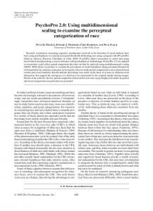
Fig. 1. Improvement on the distance estimate with node movement. (a) a sparse network. (b) If we can insert a node at A′ and a node at E ′ , then the graph becomes more rigid.

Apply the classical MDS to the distance matrix and retain the first 2 (or 3) largest eigenvalues and eigenvectors to construct a 2-D (or 3-D) local map. • Refine the local map. Using the node coordinates in the MDS solution as the initial point, a least squares minimization is performed to make the distances between nearby nodes match the measured ones. 3) Merge local maps. Local maps can be merged either sequentially or in parallel. 4) Given sufficient anchor nodes (3 or more for 2-D networks, 4 or more for 3-D networks), transform the global map to an absolute map based on the absolute positions of the anchors. •

3. M OBILE S ELF -L OCALIZATION (MSL) P ROBLEM In this section, we first introduce the mobile self-localization problem, and then discuss scenarios that generate such problems. 3.1. Mobile Self-Localization (MSL) Problem The self-localization problem for sensor networks can be formalized as follows. Given a distance graph G = hX, D, Ai where X is the set of locations of N nodes in a s-dimensional spaces (s is 2 or 3), D is a set of distance values between the nodes: dij ∈ R, and A is a set of anchor nodes, i.e., a subset of X, with cardinality m ≪ N , whose elements have known locations, find n = N − m unknown locations, X = [x1 x2 ...xn ], where xi ∈ Rs denotes the location of node i, such that |xi − xj | = dij . If A is empty or too few, only relative geolocations among nodes can be recovered. Since the range data may be noisy, this problem can be squares problem, i.e., minimizing P formalized as a least wij (|xi − xj | − dij )2 where wij are weights related to the noise levels of dij . The problem is difficult even for centralized solutions, since there is a large degree of freedom (s × n variables) when n is large. Furthermore, the solution may not be unique if the distance graph is not rigid [32]. When the connectivity is sparse, none of the existing self-localization algorithms would work well. For correct localization, one essential requirement is that the graph must be rigid, which means the existing constraints in the graph must be sufficient to determine a unique position of each node in the graph. Otherwise, there may be multiple solutions and no algorithm can guarantee correct localization.

E

4

For example, in Fig. 1-(a), node A actually can be anywhere in the circle centered at B with radius equal to |AB|. Goldenberg et. al. [33], [34] presents a detailed discussion about the conditions for a two dimensional graph to be globally rigid and introduces an algorithm to identify locally localizable points. The MDS-MAP method also assumes that the shortest path between nodes is approximately proportional to their Euclidean distance. While this may be true if the network is dense and isotropic, in the situation where a dense and isotropic network is not possible due to limited resources, this assumption is not necessarily true. For example, in Fig. 1-(a), while the shortest path between some nodes, such as B F, B E, are approximately proportional to the Euclidean distances, the shortest paths between A and D, and D and E are, however, significantly larger than their Euclidean distances. In this situation, the assumption of the MDS-MAP method is not valid anymore. The the initial position generated by MDS-MAP can be very different from the actual positions of nodes. Though there is a refinement step in the MDS-MAP algorithm, due to the existence of local minimums, it is hard for the refinement to draw the nodes to their correct positions. MDS-MAP(P) is more reliable compared with MDS-MAP due the fact it constructs local map only in a small neighborhood of each node and the local maps are patched together to get the global map. It still does not solve this problem completely. The non-proportional relation between pair-wise shortest paths and the Euclidean distances, and the non-rigidity of the network are two challenges for MDS-MAP methods. The first challenge affects the accuracy of the localization and the second one affects the correctness of the results. In some type of networks, such as mobile robotic networks, each node can move around within a certain range. For this type of networks, we can utilize the mobile capability of the nodes to get additional information about the networks, thus improve the accuracy of localization. The mobility of the sensor nodes allows us to increase the density of the network through virtual nodes. Here a virtual node represents an instant location of a mobile node during its movement. A mobile sensor node takes distance measurements to a set of nearby sensor nodes at its intermediate points along its trajectory. Each such point adds a virtual node as well as a set of distance measurements. If the number of measurements added by a virtual node is greater than the degree of freedom of the location coordinate, more constraints are added to the distance graph to make the graph more rigid and have better localization results. For example, the distance graph of Fig. 1-(a) is not rigid, which means the existing constraints in the network are not enough to unambiguously determine the positions of the nodes in it. However we can utilize the mobile capability of the nodes to get additional information about the networks, thus improving the accuracy of localization. For example, in Fig. 1-(b), suppose A moves straight to a new position A′ , and E moves to E ′ . If A′ can communicate with B, C, D, and E ′ can communicate with D, C, and F , then several new edges, AA′ (assume distance of movement can be measured), A′ B, A′ C, A′ D, E ′ D, E ′ C, E ′ F , E ′ E, shown as dashed lines in Fig. 1-(b) can be added into the network. With these new edges, the graph becomes more rigid. In general,

mobile nodes can be used to localize the whole network or turn a nonrigid network into a rigid network. With the improved shortest distance between nodes, we expect the accuracy of the MDS-MAP localization will get better. The mobile self-localization (MSL) problem can be defined as a self-localization problem in which X = Xr ∪ Xv where Xr = [x1 , x2 , ..., xn ] is a set of real node locations and Xv = [x11 , x21 , ...xs1 , x12 , ..., xs2 , x1n , ..., xsn ] is a set of virtual node locations, where xki denotes for k’th intermediate location of node i. Following are two scenarios to generate a mobile self localization problem: 1) Deploy a sparse sensor network, use one or more additional mobile sensors to localize the whole network. 2) Deploy a mobile sensor network, where all sensors are mobile, track snapshot of relative locations among these sensor nodes. In both scenarios, we may assume that a mobile sensor can measure the distance between two consecutive points in its trajectory, e.g., with an extra inertial sensor on board. Without that assumption, one less distance measurement will be added for each virtual node (e.g., AA′ in Fig. 1-(b)). For the first scenario, an extreme case is that the deployed network has no connectivity among its nodes, the only connections are between the mobile and the static nodes. Although applicationwise these are two different problems, technically they can be solved by the same type of algorithms. In this paper, we will evaluate the second scenario: full mobile self-localization problem. The algorithms developed can be applied to partial mobile sensor networks. Note that in this paper we will describe an improved MDS-MAP(P) for mobile self-localization. Other localization methods would work as well on the distance graph using added virtual nodes. Comparisons with other algorithms will be future work. In the rest of this section, we discuss how virtual nodes are generated using mobile nodes and some movement patterns we used in our simulation study. 3.2. Virtual Node Generation We assume the identification number of real nodes ranges from 1 to n, where n is the number of nodes with unknown locations in the network. A location identifier represents a unique location in space; for a real node, the location identifier is the node identifier i and for a virtual node the location identifier is ik , denoting k’th location of node i. To ensure the uniqueness of the identification numbers, the location identifiers of the virtual nodes can be easily set as n ∗ k + i. For the first position, k is equal to 1; for the second position, k is equal to 2, and so on. During the localization process, a mobile node can be in two status: Moving or Rest. A mobile node gets a new location identifier each time it comes to Rest. Only nodes in Rest participate in measuring distances. Before the localization starts, all nodes are in Rest status. At any Rest status during the movement process, including the initial position, a node will add a virtual node and corresponding distance measurements with its neighbors when there exist at least three neighbors. A general description of the process is presented below. Any

5 V2

snapshot of locations of all nodes, e.g., initial or final positions, can be considered as locations of real nodes, while other intermediate positions are considered as virtual nodes. • At the initial position or any intermediate position during the movement, a node broadcasts a message AddVirtualNode with its location identifier i to its neighbors. • When a neighbor with the location identifier j receives the AddVirtualNode message, it measures the distance dij between i and j and saves triple hi, j, dij i in its table. It then broadcasts the measurement to its neighbors. • When a node with location identifier i receives more than three measurements from its neighbors, all the measurements are stored locally, and it may continue to move to the next position. On the other hand, for a mobile node, if within certain time period after sending AddVirtualNode, it does not receive at least three measurements, it broadcasts an AbortVirtualNode with location identifier i, and continues to move to the next position. • Upon receiving an AbortVirtualNode with location identifier i, the neighbors simply delete all measurements relevant to location identifier i. In the network, each node keeps a local adjacency table hi, j, dij i, where i and j are location identifiers, and dij is the distance between these two locations. The distributed graph is the input to any localization solver. For a centralized solver, all the measurements are sent to a base station which performs the computation. In this paper, we present a distributed solution. The above protocol addresses a general case, where every node in the network is mobile. However, it can also be applied to those networks where only a subset of nodes are mobile. In these type of networks, the nodes which can not move are always in Rest status. 3.3. Movement Pattern of Mobile Nodes For mobile assistant localization, one can control the movement of mobile nodes to get better localization. In this section, we will discuss how the mobile nodes shall move in the network. The simplest way is to let each nodes move randomly. However, we may want to add some constraints to the movement. For example, we don’t want the network after the movement to be completely different from the original network, and we may want the positions of the nodes to be as close as possible to their original positions after movement. With the current technologies, robots have the capability of tracking the trajectory of their movement. Such technologies include dead reckoning [35], land mark based localziation [36], GPS [37], cooperative localization [38], or the combination of them. Such a self-tracking capability makes it possible to obtain the relative positions of the virtual nodes. Therefore, we can constrain the movement of mobile nodes. One strategy is to let the mobile nodes move in a circular way. They go out for a certain distance, start moving in a circle, and then try to move back to their original positions. However, we do not require the mobile nodes to get back to their original positions exactly since in real applications, the nodes can not move in a perfect path and some nodes may not even be able to finish moving in a circle due to obstacles.

V2 V5

V2

V2

V2

O’

V1(O)

V1(O)

V6

O’

O’

V3

O’

V1(O)

V1(O)

O’ V1(O) V3

V4 V3 Pattern 1

Pattern 2

V4 Pattern 3

V3 Pattern 4

V5

V4 Pattern 5

Fig. 2. Five example patterns of the movement of mobile nodes. This figure shows the idea cases where each node can move back to its original position. Vi |i=1:5 are the virtual nodes created at each intermediate position. O and O ′ are the original position and the position after movement respectively. V1 and O are overlapping. Ideally, mobile nodes can get back to their original positions. Therefore O ′ and O are overlapping. In real applications, however, this may not be true.

Due to the infinite ways of movement for mobile nodes, it is impossible for us to analyze every pattern of movement. In this paper, we will only evaluate five example movement patterns for mobile nodes, as shown in Fig. 2. In the first pattern, a node just goes out straight in a random direction for a certain distance d, adds a virtual node, and then moves back the same distance in the opposite direction. In the second pattern, each node goes out straight in a random direction for a certain distance, adds a virtual node, and then moves back twice the distance of d in the opposite direction, adds another virtual node, then tries move back to its original position. Three more movement patterns are also illustrated in Fig. 2. Each mobile node also adds a virtual node at its original position before the movement. For mobile robots that can track their movement trajectory, the distances between all virtual nodes added by the same mobile node can be known. Therefore, the virtual nodes together with the mobile node that creates them form a locally rigid graph when moving in the last three movement patterns. In Fig. 2, it is assumed that robots can get back to their original positions, therefore O and O’ are overlapping. In this case, the virtual nodes created at the original position are redundant. Due to noise or obstacles, O and O′ may not be overlapping. In the simulation experiment, we have also analyzed the situation. Each of the five movement patterns has its own pros and cons. Pattern 1 and 2 are much simpler than the other movement patterns. Robots that can only track the movement distance may take these patterns. These patterns also suffer less from the error in tracking the movement. But the number of virtual nodes added per movement is small. The other three movement patterns require the robots to have more advanced capability such as tracking not only the distance but also the direction of movement. Though they add more virtual nodes per movement, the error in tracking the movement may become more significant than that in the first two patterns. 4. MA-MDS-MAP(P) FOR M OBILE S ELF - LOCALIZATION In this section, we will discuss how to build the map of the network after virtual nodes are added in the way discussed in the previous section and present a mobile-assisted MDSMAP(P) algorithm, denoted as MA-MDS-MAP(P). After the movement of all nodes, there are two types of nodes in the network: one type is real nodes, the other type is virtual

6

nodes added during the movement of nodes. The virtual nodes only exist in the adjacency tables of the real nodes. There is no communication between a virtual node and any other nodes. However, the distances kept in the adjacency tables provide additional information of the network. Based on these information, more precise localization can be obtained through a mobile-assisted MDS-MAP(P) algorithm (MAMDS-MAP(P)). The details are discussed as follows: • Step 1: Each node broadcasts its local measurements in its K-hop neighborhood (K=2 in our experiments). Each node combines the adjacency tables of its neighbors with its own into a local table T . After removing the duplicated entries (entries describing the same edge), a node constructs a local graph centered at the real node (e.g., initial or final location), shown in Fig. 3-(a). Let the K-hop neighbors of the real node r be denoted by Sr . Sr contains all the real nodes within K-hop distance of r and some virtual nodes. Node r then constructs the distance matrix for nodes in Sr using only edges between nodes in Sr . The elements in the distance matrix are the shortest path between every two nodes in Sr . • Step 2: Node r builds its local relative map using the classical MDS method for nodes in Sr . The local map of a node contain the IDs and the coordinates of the nodes in Sr • Step 3: Node r refines the location of nodes, including the virtual nodes, in its local relative map via least squares minimization using the distance information in T and the coordinates from the step 2 as the initial point. Let hi, j, dij i denote the entries in T and pij denote the Euclidean distance between i and j based on their coordinates. The formulation of the minimization is X min wij (dij − pij )2 for all hi, j, dij i in T (8) i,j∈Sr

where wij is the weight for the distance between i and j. To compensate for the potential noise introduced in the movement of nodes, higher weight can be assigned to the distances between real nodes. • Step 4: Merge the local maps until all the real nodes are included in a core map, which grows by merging it with the local maps of neighboring real nodes. The local map with the maximum number of common nodes, including virtual nodes, with the core map is chosen to be merged with the core map. The merging can be done sequentially [25] or in a distributed way [26]. • Step 5: Transform the core map into an absolute map based on the absolute positions of anchors. Obviously, in this step, we only have to transform the coordinates of the real nodes, if we are not interested in movement histories. Let k be the average number of nodes, including virtual nodes, in a local map. The overall complexity for computing each local map is O(k 3 ). The total complexity for step 2 and 3 is O(k 3 n). Similar to the discussion in [25], the complexity of step 4 is O(k 3 n). For m anchors, the complexity of step 5 is O(m3 +n). So the total complexity of this MA-MDS-MAP(P) method is also O(n).

A D D’ C

B

O

E’

O

F

(a)

(b)

Fig. 3. (a) Only the real nodes and the virtual nodes, shown as non-filled circles, within two hops from the center node O are kept in the local map of O. The virtual nodes shown in gray spheres are not included because they are more than two hops away from O. (b) Node D and E move to D ′ and E ′ respectively and get into communication range of each other. The distance between them is kept in the adjacency table of both D and E.

The above presentation is based on the assumption that the nodes in the network are computationally powerful enough to construct the local maps. For the network in which the majority of nodes have limited computation capability, sending the local adjacency tables to some central nodes for constructing and merging the local maps might be the only way to localize the network. In the sequential merging approach, each node sends the local map to a central node. If efficient routing mechanism is not available, it will result in large number of messages. However, since all information is available on the central node, global refinement is possible. In the distributed merging approach presented in [26], at least three beacon nodes must broadcast their absolute coordinates to all nodes in the network. Broadcasting can be carried out very efficiently but global refinement is hard to implement in this approach. The above presentation does not consider building local maps around virtual nodes to save computation. However, we can treat virtual nodes in the same way as real nodes if each node sends its adjacent table to a central node for localization. In this scenario, the complexity in step 1, 2, and 3 will be increased. The increase will be linear with respect to the number of virtual nodes. For example, if three virtual nodes are added per movement, the complexity in the first three steps will be three times larger. The complexity of step 4 and 5, however, will not change much. An experiment in evaluating the performance when building local maps around virtual nodes is presented in section 5. 5. S IMULATION

RESULTS

5.1. Performance Comparison with Static Networks Simulation experiments have been carried out to evaluate the localization improvement after introducing movements under various network settings. We assume that distance between sensors within communication range can be measured reliably. As we know, the accuracy of the MDS-MAP method is highly dependent on the density/degree of the network. The higher the degree of each node, the more accurate the localization is. For the rest of this paper, the degree of a node refers to the number of neighbors that the node can communicate directly. The degree of a network is the average degree of nodes in it. Therefore, we would focus the experiments in evaluating the improvement of the proposed scheme in the localization of

E

7

sparse networks, whose degree is under 5. We compared the performance of MA-MDS-MAP(P) in mobile networks with MDS-MAP(P) in static networks of both uniform topology and irregular topology. The settings and results of the experiments on each type of networks are discussed below. In the following experiments, mobile nodes move in pattern 1 as shown in Fig. 2. Fig. 4 shows the experiment on a network with 200 nodes randomly positioned within a 10 * 10 field. The communication range is 1.0. To prevent the nodes from getting to too close to each other, the minimum distance between any two nodes is larger than 0.5. The average degree is 4.72. Fig. 4(a) shows the graph of the network. Fig. 4-(b), (c) show the localization errors from static localization and the mobileassisted localization respectively. The errors are shown by a line segment starting from the actual position towards the estimated one. The longer the line segments are, the larger the error is in localization. It can be seen that after incorporating the information obtained from the movement of nodes, the mean error is reduced by more than 90% and the deviation of the error is reduced by more than 80%. Fig. 5 shows the experiments on a network with 144 nodes regularly positioned within a 10 * 10 grid. There are 12 nodes in each row/column. To model the error in grid placement, the position of the nodes are adjusted by a uniformly distributed noise. The mean of the noise is 0, the range is between −0.09r and 0.09r, where r is the communication range, which is 1.0 in this experiment. The average degree is 4.39. Fig. 5-(a) shows the graph of the network. Fig. 5-(b), (c) show the localization error by using MDS-MAP(P) and MA-MDSMAP(P) respectively. It can be seen that after incorporating the information obtained from the movement of nodes, the mean of estimate error decreased from 0.162 to 0.0017, almost reduced by 99%. The standard deviation of the error decreased from 0.10585 to 0.001373, reduced by more than 98%. It is obvious that the estimate by MA-MDS-MAP(P) is significantly better. Fig. 6 and Fig. 7 show the experiments on irregular networks of C-shape topology. The localization for irregular networks is much more challenging than that for uniform networks because the error made in any step during the merging stage is easily propagated to the whole networks due to the limited paths of merging (the merging has to follow the topology of the networks). The degrees of the networks in this experiment are 3.96 and 4.12 respectively. The communication range of the nodes in both experiments is 1.0. The size of the field is 10 * 10. Fig. 6 shows the experiments with 112 nodes regularly positioned in a C-shape field. The position of each node is adjusted by the same noise as that in the experiment of a regular uniform network. As we can see from Fig. 6-(b), (c), the mean of the estimate error decreased from 0.69 to 0.0087, and the standard deviation of the error decreased from 0.50 to 0.007. Fig. 7 shows the comparison on the random C-shape network which contains 150 nodes and the communication range is 1.0. The minimum distance between any two nodes is 0.5. It can be seen that the mean of the estimate error went down from 0.28 to 0.07 and the standard deviation decreased from 0.27 to 0.035.

TABLE I T HE ERROR COMPARISON ON FOUR TYPES OF NETWORKS. F ROM LEFT TO RIGHT: RANDOM UNIFORM , REGULAR UNIFORM , REGULAR C SHAPE , AND RANDOM

mean deviation

MDS-MAP(P) MA-MDS-MAP(P) MDS-MAP(P) MA-MDS-MAP(P)

C SHAPE . 0.182 0.010 0.086 0.012

0.162 0.001 0.105 0.001

0.695 0.008 0.509 0.007

0.286 0.070 0.271 0.035

TABLE II P ERFORMANCE COMPARISON WHEN 10% NODES WITHIN COMMUNICATION RANGE CAN NOT COMMUNICATE. F ROM LEFT TO RIGHT: RANDOM UNIFORM , REGULAR UNIFORM , REGULAR RANDOM

mean deviation

MDS-MAP(P) MA-MDS-MAP(P) MDS-MAP(P) MA-MDS-MAP(P)

C- SHAPE , AND

C- SHAPE 0.529 0.002 0.329 0.001

0.158 0.001 0.097 0.001

0.607 0.019 0.364 0.017

0.224 0.021 0.196 0.012

A summary of the comparison is shown in Table I. The above experiment assumes that all nodes within communication range can communicate with each other. However, in real application, due to obstacles, the communication between nodes may be blocked. So we did another experiment to evaluate the improvement when some nodes within communication range can not communicate with each other. The settings are the same as the previous experiments except that when two nodes are within communication range, there is 10% chance that they are unable to communicate. Table II shows the result of this experiment. It can been seen that on random uniform, regular uniform, regular C-shape networks, more than 98% decrease in localization error has been achieved. On the random C-shape network, the error has been reduced by up to 90%. 5.2. Performance Comparison between With and Without Building Local Maps around Virtual Nodes As we have discussed in section 4, we can treat virtual nodes in the same way as real nodes if the localization is done on a central node. Therefore, we can also build local maps around virtual nodes. However, the time complexity will be different. We did an experiment to compare the complexities of the two scenarios. Fig. 8 shows the result. We can see there is significant difference in the time cost. Table III shows the error comparison between building local maps and not building local maps around virtual nodes. As we can see, there is no significant difference between the two ways. Therefore, in the experiments of the following sections, no local maps are built around virtual nodes. 5.3. Analysis of the Movement Patterns This experiment tries to evaluate the number of virtual nodes per movement on the accuracy of localization. If there is no noise in tracking the trajectory of mobile scenarios, the more virtual nodes added during the movement, the more accurate the localization would be. However, the noise in tracking the trajectory of movement will lead to inaccuracy of the estimates of the distances between the virtual nodes added by

8

Ground Truth: 200 points

Error of Estimation. Mean =0.18426 Standard Deviation=0.08633

Error of Estimation. Mean =0.010181 Standard Deviation=0.012601

10

10

10

9

9

9

8

8

8

7

7

7

6

6

6

5

5

5

4

4

4

3

3

3

2

2

2

1

1

1

0

0

0

1

2

3

4

5

6

7

8

9

10

0

1

2

(a) the network Fig. 4.

3

4

5

6

7

8

9

10

0

Error of Estimation. Mean =0.16285 Standard Deviation=0.10585 10

9

9

9

8

8

8

7

7

7

6

6

6

5

5

5

4

4

4

3

3

3

2

2

2

1

1

1

1

2

3

4

5

6

7

8

9

0

10

0

1

2

(a) the network

3

4

5

6

7

8

9

10

0

4

5

6

7

8

9

10

1

2

3

4

5

6

7

8

9

10

(c) MA-MDS-MAP(P)

Error comparison in a regular uniform network

Ground Truth: 112 points

Error of Estimation. Mean =0.28632 Standard Deviation=0.27169

Error of Estimation. Mean =0.070609 Standard Deviation=0.035548

10

10

9

9

9

8

8

8

7

7

7

6

6

6

5

5

5

4

4

4

3

3

3

2

2

2

1

1

1

0

0

1

2

3

4

5

6

7

8

9

10

(a) the network Fig. 6.

0

(b) MDS-MAP(P)

10

0

3

Error of Estimation. Mean =0.0017754 Standard Deviation=0.001373

10

Fig. 5.

2

Error comparison in a random uniform network

Ground Truth: 144 points

0

1

(c) MA-MDS-MAP(P)

10

0

0

(b) MDS-MAP(P)

Error comparison in a regular C-shape network

0

1

2

3

4

5

6

7

(b) MDS-MAP(P)

8

9

10

0

0

1

2

3

4

5

6

7

8

(c) MA-MDS-MAP(P)

9

10

9

Ground Truth: 150 points

Error of Estimation. Mean =0.28632 Standard Deviation=0.27169

Error of Estimation. Mean =0.070609 Standard Deviation=0.035548

10

10

10

9

9

9

8

8

8

7

7

7

6

6

6

5

5

5

4

4

4

3

3

3

2

2

2

1

1

1

0

0

0

1

2

3

4

5

6

7

8

9

10

0

(a) the network Fig. 7.

1

2

3

4

5

6

7

8

9

10

0

0

1

2

(b) MDS-MAP(P)

3

4

5

6

7

8

9

10

(c) MA-MDS-MAP(P)

Error comparison in a random C-shape network

TABLE III P ERFORMANCE COMPARISON BETWEEN BUILDING LOCAL MAPS AROUND VIRTUAL NODES , DENOTED AS

LMVN, AND NOT BUILDING LOCAL MAPS NLMVN. E ACH COLUMN SHOWS

3000

AROUND VIRTUAL NODES , DENOTED AS

F ROM LEFT TO

ARE RANDOM UNIFORM , REGULAR UNIFORM , REGULAR RANDOM

mean deviation

NLMVN LMVN NLMVN LMVN

random uniform regular uniform regular C shape random C shape

RIGHT, THE NETWORKS 2500

C- SHAPE , AND

C- SHAPE .

0.0064 0.0065 0.0054 0.0105

0.0102 0.0059 0.0093 0.0099

0.0227 0.0676 0.0236 0.0466

Time cost in seconds

THE RESULT OF ONE NETWORK .

0.0567 0.0675 0.0351 0.0400

the same node, which will in turn degrade the accuracy of the localization. Furthermore, it costs more energy and time to add more virtual nodes. Therefore, we want to know how many virtual nodes are sufficient for accurate localization. That is which movement pattern is sufficient for a sparse network. Similarly to the previous experiment, we tried on four types of network topologies: regular uniform, random uniform, regular C-shape, and random C-shape. The configuration (such as the number of nodes, the communication range, and the degree) of each network is the same as the networks discussed in the previous experiment. The localization error produced by adopting the five movement patterns are shown in Fig. 9. As we can see, the random C-shape is vibrating more than the other three topologies, but the mean error is still less than 0.07, about 7% of the communication range when two or more virtual nodes are added during the movement of each node. We can also see that with the increased number of virtual nodes per movement, localization generally gets more accurate. However, the improvement is getting less obvious as the number of virtual nodes per movement increases. Therefore, it is not necessary to add many virtual nodes per movement. Two to three virtual nodes per movement should be sufficient to get accurate localization. For network even sparser, such as networks with degree less than 4, we have to adopt the movement pattern that adds more virtual nodes. Generally speaking, if the product of the number of virtual nodes added per movement and the degree is larger than 10, the localization shall be acceptable.

2000

1500

1000

500

0

1

1.5

2

2.5 3 3.5 4 Number of samples per movement

4.5

5

Fig. 8. The time cost comparison between with and without building local maps around virtual nodes when processing on a central node. The curves of the same color reflect the same network. The curves with o are without building local maps around virtual nodes. The curves with + are with building local maps around virtual nodes.

The mean of the error in location estimate

The deviation of the error in location estimate

0.09

0.08 random uniform regular uniform regular C shape random C shape

0.08

random uniform regular uniform regular C shape random C shape

0.07

0.07 0.06 0.06 0.05 0.05 0.04 0.04 0.03 0.03 0.02 0.02 0.01

0.01

0

1

1.5

2

2.5 3 3.5 Number of samples per movement

4

(a) Mean error

4.5

5

0

1

1.5

2

2.5 3 3.5 Number of samples per movement

4

4.5

(b) Deviation of error

Fig. 9. Analysis of the influence of number of samples on the accuracy of localization.

5

10

The mean of the error in location estimate

5.4. Analysis of the Fraction of Mobile Nodes Up to now, we assume that every node in a network is mobile. For many networks, only a subset of nodes can move. Even for the network where all nodes are mobile, we may not want to let all nodes participate in the movement so as to save the energy and reduce the localization error caused by noise in tracking the movement trajectory. Furthermore the fraction of nodes participating in the movement is really dependent on the degree of the network, the acceptable accuracy of localization, and the noise in tracking the movement trajectory. If the network is sparse, then more nodes should participate in the movement. Otherwise, less nodes are needed. If accuracy requirement is higher, then more nodes should participate in the movement. The noise in tracking movement trajectory may become significant if large fraction of nodes participate in the movement. It is not our intention in this paper to find an optimal percentage for a specific type of networks. So we will just show an experiment to demonstrate that good result can be obtained if only partial nodes participate in the movement. In this experiment, we will evaluate for a network of certain degree, how many mobile nodes are sufficient for accuracy localization. We randomly created 10 networks for each type of topology and on each randomly generated network, we change the communication range, between 1.0 and 1.4, of the nodes to simulate networks with various degrees. The third movement pattern is adopted. In this experiment, each node has a probability p of participating in the movement. By evaluating the accuracy of localization at various levels of p, we can see that with a network of certain degree, how many nodes should participate in the movement to get the desired accuracy so as to avoid the unnecessary overhead in the sensor movement and error due to moving more nodes than needed. Fig. 10 shows the results of this experiment. As we can see from the figure, the higher the degree, the less mobile nodes are needed. For a network of degree higher than 6, the localization is good even with very small number of mobile nodes. For a network with degree less than 5, 40% of mobile nodes are sufficient. 5.5. Analysis of Reliability to Movement Tracking Noise Up to now, we have not considered the influence of noise on the accuracy of the localization. In real applications. there are two types of noise. One is the noise in measuring the distance between stationary nodes and mobile nodes. Since this noise is not caused by the movement of nodes, we are not going to analyze it here. The other noise is in tracking the trajectory of mobile nodes. This noise influences the distance estimates between virtual nodes and also the distance between virtual nodes and the final positions of mobile nodes. For example, in movement pattern 5, the distances |vi vj |i,j=1:5,i6=j , |vi o′ |, and |oo′ | will not be accurate due to this noise. However, it will not affect the distances between real nodes since after all nodes have finished movement, they can always measure the distances between them again. To evaluate how well the proposed algorithm adapts to the noise inherent in tracking the trajectories of mobile nodes, we carried out a set of experiments with various levels of Gaussian noise. In these

The deviation of the error in location estimate

0.5

0.35 random uniform regular uniform regular C shape random C shape

0.45

random uniform regular uniform regular C shape random C shape

0.3

0.4 0.25

0.35

0.3 0.2 0.25 0.15 0.2

0.15

0.1

0.1 0.05 0.05

0

0

0.02

0.04

0.06 0.08 0.1 Deviation of the noise

Mean error

0.12

0.14

0.16

0

0

0.02

0.04

0.06 0.08 0.1 Deviation of the noise

0.12

0.14

0.16

Standard deviation

Fig. 11. Evaluation of the effect of the noise in sensor movements. The horizon axis is the deviation of the noise. The vertical axis is the estimate error.

experiments, we adjust the final positions of the mobile nodes by accumulating all errors in the movement. For example, if a node v moves in pattern 3, then there are fours steps in the movement. Let the noise in the four steps be a set of independent vectors e1 , e2 , e3 and e4 , then the final position of v is adjusted by e1 + e2 + e3 + e4 . The noise {ei }4i=1 is determined by multiplying the expected travel distance with a two dimensional norm-distributed random vector. By adjusting the deviation of the norm distribution, we can know how robust the approach is against the tracking noise. From Fig. 10, we know the all the four types of network get pretty good results when half of the nodes are participating in the movement and movement pattern 3 is adopted. Therefore, in this experiment, we will analyze the influence of noise on networks with 50% mobile nodes and each mobile node moves in pattern 3. The mean of the noise is 0 and the deviation of the noise is from 0 to 0.15. Fig. 11 shows the results of the experiments. We can see that for the uniform network, under 6 percent of additive noise, both the mean and standard deviation of the error are less than 0.05, which is 5 percent of the communication range. For C-shape networks, we see more vibrations. However, the mean and the standard deviation are still quite small if the deviation of the noise is less than 0.03, which is 3 percent of the communication range. 6. C ONCLUSION In this paper, we proposed a mobile assisted localization method based on multi-dimensional scaling for robotic sensor networks to solve the self-localization problem. The MDSMAP(P) method highly depends on the degree of the network, which leads to poor performance in sparse networks. Based on the fact that robotic sensors in a mobile network have limited mobile capability, in the proposed approach, more information is obtained by moving the sensors around and adding virtual nodes during the movement. The distances between virtual nodes and real nodes are kept in adjacency tables. Virtual nodes are incorporated in building and merging the local maps. Evaluation of the performance of the proposed approach is carried out on four types of networks: random uniform, random C-shape, regular uniform, and regular C-shape. The results have shown significant improvement over the MDSMAP(P) approach on static low-degree networks. In the future, we are going to study the cases where only one or a small

11

The mean of the error in location estimate

The mean of the error in location estimate

0.2

0.14 average degree=4.719 average degree=5.752 average degree=6.952 average degree=8.234

0.18

average degree=4.3181 average degree=5.4042 average degree=6.4111 average degree=6.9167

0.12

0.16 0.1

0.14

0.12 0.08 0.1 0.06 0.08

0.06

0.04

0.04 0.02 0.02

0

0

0.1

0.2

0.3 0.4 0.5 0.6 0.7 Fraction of nodes moving in localization

0.8

0.9

1

0

0

0.1

0.2

Random uniform

0.3 0.4 0.5 0.6 0.7 Fraction of nodes moving in localization

0.8

0.9

1

Regular uniform

The mean of the error in location estimate

The mean of the error in location estimate

0.45

0.5 average degree=4.49 average degree=5.4138 average degree=6.5125 average degree=7.72

0.4

average degree=4.0161 average degree=4.9536 average degree=5.8339 average degree=6.2821

0.45

0.4

0.35

0.35 0.3 0.3 0.25 0.25 0.2 0.2 0.15 0.15 0.1

0.1

0.05

0

0.05

0

0.1

0.2

0.3 0.4 0.5 0.6 0.7 Fraction of nodes moving in localization

0.8

0.9

1

0

0

0.1

0.2

Random C-shape

0.3 0.4 0.5 0.6 0.7 Fraction of nodes moving in localization

0.8

0.9

1

Regular C-shape

The deviation of the error in location estimate

The deviation of the error in location estimate

0.25

0.12 average degree=4.719 average degree=5.752 average degree=6.952 average degree=8.234

average degree=4.3181 average degree=5.4042 average degree=6.4111 average degree=6.9167

0.1

0.2

0.08 0.15

0.06

0.1 0.04

0.05 0.02

0

0

0.1

0.2

0.3 0.4 0.5 0.6 0.7 Fraction of nodes moving in localization

0.8

0.9

1

0

0

0.1

0.2

Random uniform

0.8

0.9

1

Regular uniform

The deviation of the error in location estimate

The deviation of the error in location estimate

0.35

0.35 average degree=4.49 average degree=5.4138 average degree=6.5125 average degree=7.72

0.3

0.25

0.2

0.2

0.15

0.15

0.1

0.1

0.05

0.05

0

0.1

0.2

0.3 0.4 0.5 0.6 0.7 Fraction of nodes moving in localization

Random C-shape

0.8

0.9

average degree=4.0161 average degree=4.9536 average degree=5.8339 average degree=6.2821

0.3

0.25

0

0.3 0.4 0.5 0.6 0.7 Fraction of nodes moving in localization

1

0

0

0.1

0.2

0.3 0.4 0.5 0.6 0.7 Fraction of nodes moving in localization

0.8

0.9

1

Regular C-shape

Fig. 10. The localization error with respect to the fraction of mobile nodes on networks of four topologies: random uniform, regular uniform, random C-shape and regular C-shape. The first two rows show the mean of the error and second two rows show the standard deviation of the error.

12

number of mobile nodes that are equipped with or without motion sensors. We will also compare the performance of different localization schemes, such as SDP and isomap, for mobile self localization. ACKNOWLEDGMENT We give special thanks to Professor Yi Shang in the University of Missouri-Columbia for kindly sharing with us the Matlab simulation code. R EFERENCES [1] I. Akyildiz, W. Su, Y. Sankarasubramaniam, and E. Cayirci. A survey on sensor networks. IEEE Commun. Mag., 40:102–114, 2002. [2] A. Mainwaring, J. Polastre, R. Szewczyh, D. Culler, and J. Anderson. Wireless sensor networks for habitat monitoring. In Proceedings of Wireless Sensor Network and Applications, 2002. [3] S. N. Simic and S. Sastry. Distributed environmental monitoring using random sensor networks. In Proceedings of the 2nd International Workshop on Information Processing in Sensor Networks, pages 582– 592, 2003. [4] K. W. Kolodziej and J. Hjelm. Local Positioning Systems: LBS Applications and Services. CRC Press, Taylor & Francis Group, 2006. [5] F. Zhao and L. Guibas. Wireless Sensor Networks: An Information Processing Approach. Elsevier and Morgan Kaufmann Publishers, 2004. [6] C. Savarese, J.M. Rabaey, and J. Beutel. Locationing in distributed ad hoc wireless sensor networks. In Proc. 2001 Int’l Conf. Acoustics, Speech, and Signal Processing (ICASSP 2001), volume 4, pages 2037– 2040, May 2001. [7] N. Bulusu, J. Heidemann, and D. Estrin. GPS-less low cost outdoor localization for very small devices. Technical Report 00-729, Computer science department,University of Southern California, Los Angles, CA, 2000. [8] X. Nguyen, M.I. Jordan, and B. Sinopli. A kernel-based learning approach to ad hoc sensor network localization. ACM Transactions on Sensor Networks, 1(1):134–152, 2005. [9] J. Beutel. Master Thesis, Geolocation in a PicoRadio Environment. UC Berkeley, 1999. [10] A. Savvides, C. C. Han, and M. Strivastava. Dynamic fine-grained localization in ad-hoc networks of sensors. In ACM SIGMOBILE, 2001. [11] T. He, C. Huang, B.M. Blum, J.A. Stankovic, and T. Abdelzaher. Range-free localization schemes for large scale sensor networks. In MobiCom’03, 2003. [12] R. L. Moses, D. Krishnamurthy, and R. Patterson. A self-localization method for wireless sensor networks. Journal on Applied Signal Processing, 2003(4):148 – 158, March 2003. [13] N. Patwari, J. N. Ash, A. O. Hero, R. Moses, and N. S. Correal. Locating the nodes. IEEE Signal Processing Magazine, 54, July 2005. [14] A. Savvides, W. L. Garber, R. L. Moses, and M. B. Srivastava. An analysis of error inducing parameters in multihop sensor node localization. IEEE Transactions on Mobile Computing, 4(6), November/December 2005. [15] H. Lim and J. Hou. Localization for anisotropic sensor networks. In Proc. IEEE InfoComm05, Miami, FL, 2005. [16] J. Cortes, S. Martinez, T. Karatas, and F. Bullo. Coverage control for mobile sensing networks. In IEEE Trasactions on Robotics and Automation, pages 243–255, 2004. [17] Guiling Wang, Guohong Cao, and T. La Porta. Movement-assisted sensor deployment. IEEE INFOCOM 2004, vol.4:2469–2479, 2004. [18] J. R. Spletzer. Sensor Fusion Techniques for Cooperative Localization in Robot Teams. PhD thesis, University of Pennsylvania, 2003. [19] S. Tilak, V. Kolar, N. B. Abu-Ghazaleh, and K. D. Kang. ”dynamic localization control for mobile sensor networks”. In Proceedings of IEEE International Workshop on Strategies for Energy Efficiency in Ad Hoc and Sensor Networks, April 7-9 2005. [20] L. Hu and D. Evans. Localization for mobile sensor networks. In Proceedings of MobiCom’04, pages 45–57, 2004. [21] C. Taylor, A. Rahimi, and J. Bachrach. Simulatenous localization, calibration and tracking in an ad hoc sensor network. In 5th International Conference on Information Processing in Sensor Networks (IPSN06), 2006. [22] N. B. Priyantha, H. Balakrishnan, E. D. Demaine, and S. Teller. Mobileassisted localization in wireless sensor networks. In IEEE Conference on Computer Communications (InfoCom05), 2005.

[23] P. N. Pathirana, N. Bulusu, A. Savkin, and S. Jha. Node localization using mobile robots in delay-tolerant sensor networks. IEEE Transactions on Mobile Computing, 4(4), July/August 2005. [24] C. Wang, Y. Ding, and L. Xiao. Virtual ruler: Mobile beacon based distance measurements for indoor sensor localization. In The Third International Conference on Mobile Ad-hoc and Sensor Systems (MASS06), 2006. [25] Y. Shang and W. Ruml. Improved mds-based localization. In Proceedings of IEEE InfoCom’04, 2004. [26] Y. Shang, W. Ruml, and M. Fromherz. Positioning using local maps. ”Ad Hoc Networks” Journal of Elsevier, 4:240–253, 2006. [27] P. Biswas and Y. Ye. Semidefinite programming for ad hoc wireless sensor network localization. In ACM/IEEE Conference Information Processing in Sensor Networks, 2004. [28] X. Ji and H. Zha. Sensor positioning in wireless ad-hoc sensor networks using multidimentional scaling. In IEEE Conference on Computer Communications (InfoCom04), 2004. [29] J.A. Costa, N. Patwari, and A. Hero. Distributed weightedmultidimentional scaling for node localization in sensor networks. ACM Transactions on Sensor Networks, 2(1), February 2006. [30] J. B. Kruskal and Wish. M. Multidimensional Scaling. Sage Publications, Beverly Hills, CA, 1977. [31] Young. F. W. and Hamer. R. M. Theorv and Applications of Multidimensional Scaling. Eribaum Associates, Hillsdale, NJ, 1994. [32] A. So and Y. Ye. Theory of semidefinite programming for sensor network localization. In SODA05, 2005. [33] T. Eren, O.K. Goldenberg, W. Whiteley, A.S. Yang, Y.R.; Morse, B.D.O. Anderson, and P.N.; Belhumeur. Rigidity, computation, and randomization in network localization. In Proceedings of IEEE INFOCOM 2004, Twenty-third AnnualJoint Conference of the IEEE Computer and Communications Societies, volume 4, pages 2673 – 2684, March 2004. [34] D.K. Goldenberg, A. Krishnamurthy, W.C. Maness, Y.R. Yang, A. Young, A.S. Morse, and A. Savvides. Network localization in partially localizable networks. In Proceedings of IEEEINFOCOM 2005, 24th Annual Joint Conference of the IEEE Computer and Communications Societies., pages 313 – 326, March 2005. [35] B. Yamauchi. Mobile robot localization in dynamic environments using dead reckoning and evidence grids. In Proceedings of the 1996 IEEE Interational Conference on Robotics and Automation, pages 1401 – 1406, 1996. [36] Gijeong Jang; Sungho Kim; Wangheon Lee; Inso Kweon. Robust selflocalization of mobile robots using artificial and natural landmarks. In Proceedings of 2003 IEEE International Sysmposium on Computational Intelligence in Robotics and Automation, pages 412 – 417, 2003. [37] F. Capezio, A. Sgorbissa, and R. Zaccaria. Gps-based localization for a surveillance ugv in outdoor areas. In Proceedings of the Fifth International Workshop on Robot Motion andControl, pages 157 – 162, 2005. [38] A.I. Mourikis and S.I. Roumeliotis. Performance analysis of multirobot cooperative localization. IEEE Transactions on Robotics, 22(4):666 – 681, 2006.

Chang-Hua Wu Dr. Wu obtained his B.A. and M.S. degrees from Hangzhou Dianzi University, formerly Hangzhou Institute of Electronic Engineering (HZIEE) in 1998 and 2001 respectively. As a graduate student, he conducted research in the recognition and generation of facial expressions. In 2001, he enrolled in the Ph.D. program of the computer science department at Illinios Institute of Technology and got the Ph.D. degree in 2005. He joined the department of science and mathematics of Kettering University as an Assistant Professor in Sept. 2005. Dr. Wu is a professional member of IEEE and ACM, and has served as a reviewer for multiple conferences. His current research area includes medical image analysis, computer vision, intelligent robot, image retrieval and mobile networks.

13

Weihua Sheng Weihua Sheng received his Ph.D degree in Electrical and Computer Engineering from Michigan State University in May 2002. He obtained his M.S and B.S. degrees in Electrical Engineering from Zhejiang University, China in 1997 and 1994, respectively. Currently he is an assistant professor in the School of Electrical and Computer Engineering at Oklahoma State University. He has been involved in research projects funded by Ford Motor Company and NSF. His research work has resulted in one patent in US and more than 50 papers in major journals and international conferences in robotics and automation. His current research interests include distributed robotic systems, mobile wireless sensor networks, process planning for advanced manufacturing technologies and embedded computing. He is a member of IEEE Robotics and Automation Society, IEEE Computer Society and ACM.

Ying Zhang Dr. Ying Zhang is a member of research staff at Palo Alto Research Center (PARC). She obtained her PhD in Computer Science from University of British Columbia in 1994. Dr. Zhangs current research interests are in sensor/actuator networks and embedded control architectures. She has led software architecture development for modular reconfigurable robots at PARC and has been working on constraintbased routing and localization on sensor networks. Dr. Zhang is the information director of the ACM Transaction on Sensor Networks, and has served as TPC, guest editor, and NSF review panelist on sensor networks.